Download

1 / 25
250 likes | 380 Vues
Population dynamics of aquatic top predators: effects of harvesting regimes and environmental factors. Project leader: Professor Nils Chr. Stenseth Post-doc: Dr. Scient. (PhD) Thrond O Haugen. Who is involved?. Centre for Ecology and Hydrology PhD Ian Winfield University of Oslo

E N D
Population dynamics of aquatic top predators: effects of harvesting regimes and environmental factors Project leader: Professor Nils Chr. Stenseth Post-doc: Dr. Scient. (PhD) Thrond O Haugen
Who is involved? • Centre for Ecology and Hydrology • PhD Ian Winfield • University of Oslo • Professor Leif Asbjørn Vøllestad • PhD Per Aass (at the Zoological Museum) • Mangement institutions • Tore Qvenild (fishery manager, Hedmark county) • MSc Ola Hegge (fishery manger Oppland county) • Norwegian Institute of Water Research (NIVA)
Project objectives • Increase knowledge on population dynamics of aquatic top predators • How is population dynamics affected by changes in: • Abiotic conditions (temperature and eutrophication) • Biotic conditions (prey abundance, density) • Harvesting regimes (qualitative and quantitative) • Reliable estimates of demographic rates: • Survival (age, stage, sex specific, environment-specific, density-specific, basin specific) • Recruitment (population growth rate)
From fate diagrams… Alive and recaptured p Alive f 1-p Alive and not recaptured Marked and released 1-f Dead or emigrated • is apparent survival (open systems) pis probability of recapture
f1 f2 f3 f4 f5 ...tocapture historyandsurvival estimats CaptureMark Release Capture occations Time interval p2 p3 p4 p5 p6 Capture history: 100100, with probability: f1(1-p2)f2(1-p3)f3p4c4 c4 is the probability of not being recaptured after 4th capture occation [= (1-f4)+(1-p5)f4(1- p6f5)] Parameters areestimatedby maximum likelihood method
Maximum log-likelihood estimation(MLE) • Under the assumption of mutually exclusive capture histories probabilities of unique capture histories may be estimated • independence of fates and identity of rates among individuals • Statistical likelihood of a data set is the product of capture histories over all capture histories observed • Maximizes the log-likelihood for the estimator q of the vector q containing all identifiable parameters [i.e. maxlnL(q)] ^ ^
MLE: an example t1 t2 t3 b3 f1 f2 Para- meters p1 p2 p3 Likelihood: L= (f1p2b3)X111[f1p2(1-b3)]X110[f1 (1-p2)b3]X101 (c1)X100 lnL(f1, p2, b3)= 4ln(f1p2b3)+7ln[f1p2(1-b3)]+2ln[f1 (1-p2)b3]+9ln(c1)
Based on log-likelihood-ratio tests (LRT) For nested models only LRT = -2lnL(q0)-(-2lnL(q)) ~c2 with np-rdf Problems with multiple testing Akaike Information Criterion (AIC) No testing involved AIC = -2lnL + 2*np (choose the lowest) May not converge to one model only Biological a priori knowledge should guide the formation of hypotheses and the selection of models! Model selection q0= parameter vector for reduced model q = parameter vector for full model
Combination fate diagram p Alive and recaptured F Alive and still present 1-p Alive and not recaptured Alive S 1-F Alive and left the system Capture Mark Release r Dead and reported 1-S Dead 1-r Dead and not reported
F1 F2 F3 F4 F5 S1 S2 S3 S4 p1 p2 p3 p4 p5 r1 r2 r3 r4 J F M A M J J A S O N D Joint analysis of dead recoveries and live encounters—non-Brownie parameterisation St = probability of survival from time t to t+1(survival rate) rt = probability of being found dead and reported during the t to t+1 interval (recovery probability) Ft= probability at tof remaining in the sampling area to t+1 | alive at t (fidelity rate) pt = probability of recapture at time t | alive and in sampling area (recapture rate)
The data series • Trout from Mjøsa (n = 7002; 1966–2001); pike from Windermere (n = 5560; 1949–2001) • Combined data • Recoveries (dead) and recaptures • Continous and experimental recaptures • Good environmental data (covariates) • Eutrophication, temperature, prey abundance • Fishing effort • Multiple recaptures • 57.9 % of the pike have been recaptured once or more • 38.1 % for Mjøsa trout • Constraints: • Allmost exclusively mature fish (all for the trout)
J F M A M J J A S O N D Windermere Dead recoveries – natural causes Dead recoveries from gill nets Marking and recaptures Marking and some recaptures by use of traps and seines Dead recoveries from gill nets – Experimental fisheries only Dead recoveries from anglers Dead recoveries – natural causes Dead recoveries from gill nets and anglers Marking and recaptures by use of trap in a fish ladder Mjøsa
Addressed questions • Are there temporal inter- and intra-annual trends in survival rates? • Does gill netting affect the survival rates? • What is the relative contribution from anglers and gill netting to the total mortality? • Does size at marking affect the survival rates? • Does age affect survival rates? • Does sex affect the survival rates?
Quarterly survival rates in Windermere pike for 1954–1963 cohorts Tagging cohorts analysed
Late-autumn survival vs rest of the year Tagging cohorts analysed
Does sex affect survival? Tagging cohorts analysed
Age-structured model combined with annual summer survival for spawning age > 4
Challenges to come • How sensitive are the parameter estimates to changes in the discretisation policy • GOF must be performed! • Estimating c-hat • Do the entire time series for Windermere