Download
1 / 45
450 likes | 726 Vues
Introduction to Computer Science 2. Lecture 12: Sorting (Part 2). Prof. Neeraj Suri Constantin S ârbu Overview: Heapsort Proxmap Sort Counting Sort. Recap: Sorting. Fundamental problem in computer science Methods already presented: Selection sort Insertion sort Bubblesort

E N D
Introduction to Computer Science 2 Lecture 12: Sorting (Part 2) Prof. Neeraj Suri Constantin Sârbu Overview: Heapsort Proxmap Sort Counting Sort
Recap: Sorting • Fundamental problem in computer science • Methods already presented: • Selection sort • Insertion sort • Bubblesort • Shellsort ( O(n1,2) ) • Quicksort ( O(n•log n) ) • All have complexity O(n2) • Better: Quicksort (divide and conquer) with complexity O(n•log2n) on average
Sorting methods: Overview sorting themes HW supported parallel sort:Systolic arrays address calculation sorting:Proxmapsort, Radixsort, Counting sort comparison-based sorting transposition sorting:Bubblesort O(n2) Insert and keep sorted:Insertion sort, Tree sort diminishing incrementsort: Shellsort priority queue sorting:Selection sort, heapsort O(n•log n) divide and conquer:Quicksort, Mergesort
The Sorting Problem • Given: • A list of n elements (or data records) E1, E2, ... , En • Each element Ei contains a key Ki • We need: • “a sorted series”, more exactly: • A permutation (reordering) of numbers 1 to n, such that if the series is sorted according to , then K(1) K(2) ... K(n)
Sorting: Basic Framework • Java-Class: class Element { int key; /* sorting key */ Info info; /* real information */ } • The elements are stored in an array : Element L[n-1]; • The cost: • The number of comparisons (of keys) • The number of swaps (of elements in the array)
Logarithmic Sorting method • Sorting algorithms, that have complexity O(n2), are not useable for large number of keys • Even the costs of the Shellsort rise fast with the n, O(n1.25). • We already know a sorting method with complexity O(n log2n): Quicksort • But there are others methods of sorting in this class, that are based on tree structures introduced in the previous lecture
Merge Sort • Important sorting algorithm • Based on “Divide and Conquer” • John Van Neuman (1945) • mergesort(array): • Divide the array in two (equal) halves • Run mergesort on both halves • Merge the result
8 4 6 2 7 1 3 5 8 4 3 5 6 2 7 1 4 3 5 6 2 7 1 8 Mergesort 6 2 7 1 8 4 3 5
1 2 3 4 5 6 7 8 3 4 1 2 6 7 5 8 4 8 3 5 2 6 1 7 Mergesort 4 3 5 6 2 7 1 8
Mergesort • Complexity • Divide: O(1) • Recursion: 2T(n/2) • Merging: O(n) • Total: n log n • Mergesort used in Perl (after 5.8), Java 1.5
Heapsort • Goal: Sorting algorithm, that works in O(n log2n) without additional memory requirements • Heapsort: classic sorting method (1964 J.W.J. William) • The algorithm is based on a binary tree, the Heap, and consists of two phase: • First build of the Heap • Progressively editing the Heap to sort it
Heap • Definition: A binary tree B with n nodes is a Heap of size n, when: • B is nearly complete • The keys are sorted in such a way, that for each node i, Ki Kj, where node j is the parent node of the node i. • Important: a Heap is a nearly complete binary tree but not a binary search tree. Examples for Heaps
Heap properties • In one Heap each subtree is a Heap • In a Heap the biggest element is in the root • No Heaps (violation of the first or of the second condition):
The Heapsort Algorithm • The construction of the Heap from the input sequence • input sequence: 2, 9, 56, 77, 12, 13, 96, 17, 56, 44 • The initial tree, not a Heap just yet: Reminder: Array position n 2n 2n+1
The Heap Construction • Fulfill the heap conditions by swapping leaves
The Heap Construction • Fulfill the heap conditions by swapping leaves
The Heap Construction • Fulfill the heap conditions by swapping leaves
The Heap Construction (2) • Now: Heap conditions fulfilled, finish Heap.
Sorting Procedure • After the construction of the heap follows the sorting procedure: • Extract the biggest element from the root, place it on the corresponding position (the “last” position) • Mark the elements that will be separated by the rest of the tree • Fulfill the heap conditions again Initial Heap Heap after the biggest element was extracted and marked
Result • The tree can be stored in a sequential representation without additional memory (no holes) • The sorted sequence is obtained after the biggest element was extracted and the Heap conditions where fulfilled n times • Heap conditions fulfillment need O(log2n) time: • Analog with the transformation of other trees with limited transformation complexity • Fulfill the Heap conditions each time a tree was constructed • The complexity is proportional with the maximal length of the path to a leave. So the height of the tree. • Total run time O(n log2n) • Can we do any better?
Lower Bounds on Sorting • What we’ve seen so far is comparison sort • Based on comparing elements • Assume only comparisons cost • Still we have a lower bound of O(n log n)! • But we can do better … • Proxmapsort • Counting sort
Lower Bounds on Sorting • We must somehow compare all elements to get the sorting correct • What is the minimum number of comparisons that needs to be done? • Idea: we must do pair-wise comparisons • We could build a binary decision tree …
a1:a2 > ≤ a2:a3 a1:a3 ≤ > ≤ > a2,a1,a3 a1,a2,a3 a1:a3 a2:a3 ≤ > ≤ > a1,a3,a2 a3,a1,a2 a2,a3,a1 a3,a2,a1 Lower Bounds on Sorting
a1:a2 > ≤ a2:a3 a1:a3 ≤ > ≤ > a2,a1,a3 a1,a2,a3 a1:a3 a2:a3 ≤ > ≤ > a1,a3,a2 a3,a1,a2 a2,a3,a1 a3,a2,a1 Lower Bounds on Sorting • What is the maximum number of comparisons? • The height of the tree! • Maximum number of nodes is n! • All permutations of n numbers • Complete binary tree has 2h leaves 2h≥ n! h ≥ log (n!)
Linear Sorting • Idea: Do not base the sorting on comparisons! • Proxmap sort • Counting sort
Sorting with address computation(Proxmap Sort) • Basic idea (the same as counting sort): • With the help of an address computation, i.e. a mapping f(K)= address, a key is shifted in the first pass to the proximity of the final destination. • The final sorting is done using local fine grained sorting Steps: • Definition of the mapping • Assignment of the neighbors • The interchange of the keys • Fine grained sorting
Example • Mapping: MapKey(K) = K
Possible Improvements No linked lists but reserve areas in Array • One passes the array once and adopt MapKey • One count the frequency of the mapped values (hit counts): • H[0] = 1 • H[1] = 3 • H[2] = 0 etc. • Reserve areas in Array, that are proportional with the frequency: • 0-Region starts at A[0] • 1-Region starts at A[1] • 3-Region starts at A[4] etc.
Possible Improvements (2) Placing the keys: • Placing in a second Array: • easier and faster, but demands double memory • In situ placing • more complicated (key marking) and slower, but demands only one array Better mapping: • Similar problem with hashing (later) • Must find coding for non-numeric keys • Mapping possible without generating collisions • Each collision means a local sorting (for example insertion sort)
Execution Time The worst case • All the keys are mapped to the same address • degenerate to insertion sort, O(n2) • The best case • Perfect mapping, i.e. each key will be mapped to a different address • One pass to apply MapKey and to generate hit counts • One pass to generate the ProxMap • One pass to copy the key from the input array in the final position • One pass of the ProxMap • Total O(n) !!!
Execution Time Average case: • We divide n keys in areas with c keys and obtain n/c areas • Each area must be sorted with insertion sort with O(c2) • Total cost is (n/c) O(c2), so (n/c) (ac2 + bc + c) = nac + nb + nd/c • For c << n is then O(n) • Linear execution time for Proxmap Sort can be experimentally verified
Counting Sort • Assumption: sort n integers in the range 0..k • Idea: find the number of elements less than a number i, then we know the final position of i • Needed: 3 arrays • A[1..n]: the input • B[1..n]: the output • C[1..k]: help array (initialized to 0)
Counting Sort 5 2 7 1 2 4 3 5 A Step 1: Count the occurrences of the elements, store in C 1 2 3 4 5 6 7 0 1 1 1 2 1 1 2 C Step 2: Count the number of elements less than or equal to i, update C 1 2 3 4 5 6 7 7 8 1 1 3 4 5 7 C
Counting Sort 5 2 7 1 2 4 3 5 A 1 2 3 4 5 6 7 7 8 1 1 3 4 5 7 C Step 3: For each element A[n..1], place it at B[C[i]] and do C[i]-- 1 2 3 4 5 6 7 8 B
Counting Sort 5 2 7 1 2 4 3 5 A 1 2 3 4 5 6 7 7 8 1 1 3 4 5 6 C Step 3: For each element A[n..1], place it at B[C[i]] and do C[i]-- 1 2 3 4 5 6 7 8 5 B
Counting Sort 5 2 7 1 2 4 3 5 A 1 2 3 4 5 6 7 7 8 1 1 3 3 5 6 C Step 3: For each element A[n..1], place it at B[C[i]] and do C[i]-- 1 2 3 4 5 6 7 8 3 5 B
Counting Sort 5 2 7 1 2 4 3 5 A 1 2 3 4 5 6 7 7 8 1 1 3 3 4 6 C Step 3: For each element A[n..1], place it at B[C[i]] and do C[i]-- 1 2 3 4 5 6 7 8 3 4 5 B
Counting Sort 5 2 7 1 2 4 3 5 A 1 2 3 4 5 6 7 7 8 1 1 2 3 4 6 C Step 3: For each element A[n..1], place it at B[C[i]] and do C[i]-- 1 2 3 4 5 6 7 8 2 3 4 5 B
Counting Sort 5 2 7 1 2 4 3 5 A 1 2 3 4 5 6 7 7 8 0 1 2 3 4 6 C Step 3: For each element A[n..1], place it at B[C[i]] and do C[i]-- 1 2 3 4 5 6 7 8 1 2 3 4 5 B
Counting Sort 5 2 7 1 2 4 3 5 A 1 2 3 4 5 6 7 7 7 0 1 2 3 4 6 C Step 3: For each element A[n..1], place it at B[C[i]] and do C[i]-- 1 2 3 4 5 6 7 8 1 2 3 4 5 7 B
Counting Sort 5 2 7 1 2 4 3 5 A 1 2 3 4 5 6 7 7 7 1 0 1 3 4 6 C Step 3: For each element A[n..1], place it at B[C[i]] and do C[i]-- 1 2 3 4 5 6 7 8 1 2 2 3 4 5 7 B
Counting Sort 5 2 7 1 2 4 3 5 A 1 2 3 4 5 6 7 7 7 1 0 1 3 4 5 C Step 3: For each element A[n..1], place it at B[C[i]] and do C[i]-- 1 2 3 4 5 6 7 8 1 2 2 3 4 5 5 7 B
Counting Sort • Costs: • Step 1 in Θ(n) [count occurrences] • Step 2 in Θ(k) [sum up the elements ≤ i] • Step 3 in Θ(n) [place the elements in B] • Overall Θ(k+n) • Usually in practice k=O(n) so • Complexity is Θ(n) • Note the stability of the sorting order! • Equal elements appear in the same order as in the input