Download
1 / 25
440 likes | 1.32k Vues
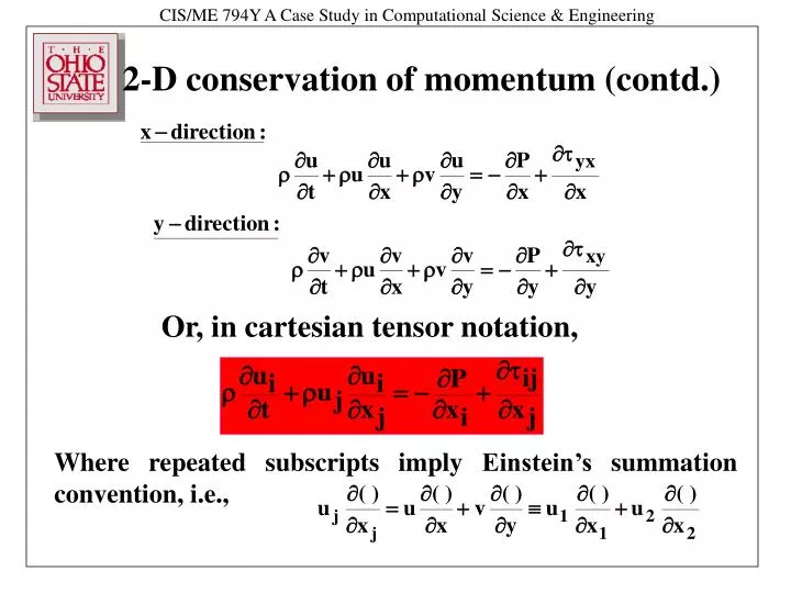
2-D conservation of momentum (contd.). Or, in cartesian tensor notation,. Where repeated subscripts imply Einstein’s summation convention, i.e.,. Conservation of momentum (contd.):.

E N D
2-D conservation of momentum (contd.) Or, in cartesian tensor notation, Where repeated subscripts imply Einstein’s summation convention, i.e.,
Conservation of momentum (contd.): The shear stress tij is related to the rate of strain (i.e., spatial derivatives of velocity components) via the following constitutive equation (which holds for Newtonian fluids), where m is called the coefficient of dynamic viscosity (a measure of internal friction within a fluid): Deduction of this constitutive equation is beyond the scope of this class. Substituting for tij in the momentum conservation equations yields:
Navier-Stokes equations for 2-D, compressible flow The conservation of mass and momentum equations for a Newtonian fluid are known as the Navier-Stokes equations. In 2-D, they are:
Navier-Stokes equations for 2-D, compressible flow in Conservative Form The Navier-Stokes equations can be re-written using the chain-rule for differentiation and the conservation of mass equation, as: (1) (2) (3)
Conservation of energy and species The additional governing equations for conservation of energy and species are: (4) (5)
Summary for 2-D compressible flow • UNKNOWNS: r, u, v, T, P, ni N+5, for N species • EQUATIONS: • Navier-Stokes equations (3 equations: conservation of mass and conservation of momentum in x and y directions) • Conservation of Energy (1 equation) • Conservation of Species ((N-1) equations for n species) • Ideal gas equation of state (1 equation) • Definition of density: (1 equation)
Non-dimensionalize the 2-D governing equations exactly as we did the quasi 1-D governing equations. Take geometry into account. For example, Extension of LBI method to 2-D flows Outer Body Center Body
Let ri(x) represent the inner boundary, where x is measured along the flow direction. Let ro(x) represent the outer boundary, where x is along the flow direction. ri(x) ro(x)
The real domain is then transformed into a rectangular computational domain, using coordinate transformation: y or r x x h
The coordinate transformation is given by: The governing equations are then transformed:
Or, and etc.
This will result in a PDE with h and x as the independent variables; for example, Recall that for quasi 1-D flow, we had equations of the form
Applying the same procedure to our transformed 2-D problem would yield: Recall that after linearization of the quasi 1-D problem, the resulting matrix system was:
Now, in 2-D, the linearization procedure will result in: Where each Fi, Gi, Hi are themselves block tri-diagonal systems as in the quasi 1-D problem. In other words, etc.
At this point, we have a choice: We can solve the full system as is, i.e. an (M+N)x(M+N) linear sparse system. Or We can split the operator and apply the Alternating Direction Implicit (ADI) method to reduce the 2-D operator to a product of 1-D operators in each of the coordinate directions and solve each alternately, at each time step.
Recall that after Crank-Nicolson differencing in time, linearization, and discretization of the spatial derivatives, we have: Split the operator by implicit factorization, approximate to either order (Dt) or (Dt)2 as in the original discretization errors. Douglas-Gunn ADI scheme
Note that: Thus, operator splitting yields: Defining , we have:
Note that now, the solution of and is identical to solving two equivalent quasi 1-D problems in each of the coordinate directions x and h. The Douglas-Gunn ADI scheme after implicit factorization can be shown to be unconditionally stable in 3-D as well as long as the convective term is absent, but is conditionally stable with the convective term present.
The conditional stability of this scheme worsens and may vanish if there are periodic boundary conditions. A virtue of the Douglas-Gunn ADI approach is that the same boundary conditions used for can be be used for W. This is a result of consistent splitting of the operator. Other operator splitting schemes exist that are inconsistent - the same BCs used for cannot be used for W.
In the present case study problem, our governing equations are of the form: Applying the LBI method to this equation yields: The Douglas-Gunn operator splitting then yields:
Still, no matrix inversion is required. The solution procedure can be implemented as follows: Set solve for W in “xinv” Next, solve for fn+1 - fn in “rinv”
10,000 time steps at Dt = 10-4 (non-dimensional) then for 100,000 time steps at Dt = 2x10⁻³ (non-dimensional). Lref = 1 cm.; Pref = 1.013 x 10⁵ Pa; Tref = 300 K 260 x 50 grid (x * r) Artificial Dissipation: or Key features