Download
1 / 59
650 likes | 1.04k Vues
Economic Analysis for Business Session IV: Market Forces of Supply and Demand-I. Instructor Sandeep Basnyat 9841892281 Sandeep_basnyat@yahoo.com. 0. Markets and Competition. A market is a group of buyers and sellers of a particular product.

E N D
Economic Analysis for BusinessSession IV: Market Forces of Supply and Demand-I InstructorSandeep Basnyat 9841892281 Sandeep_basnyat@yahoo.com
0 Markets and Competition • A market is a group of buyers and sellers of a particular product. • A competitive market is one with many buyers and sellers, each has a negligible effect on price. • A perfectly competitive market: • all goods exactly the same • buyers & sellers so numerous that no one can affect market price – each is a “price taker” • In this chapter, we assume markets are perfectly competitive. CHAPTER 4 THE MARKET FORCES OF SUPPLY AND DEMAND
0 Demand • Demand comes from the behavior of buyers. • The quantity demanded of any good is the amount of the good that buyers are willing and able to purchase. • Law of demand: the claim that the quantity demanded of a good falls when the price of the good rises, other things equal.
0 The Demand Schedule • Demand schedule: A table that shows the relationship between the price of a good and the quantity demanded. • Example: Helen’s demand for lattes. • Notice that Helen’s preferences obey the Law of Demand. CHAPTER 4 THE MARKET FORCES OF SUPPLY AND DEMAND
Helen’s Demand Schedule & Curve Price of Lattes Quantity of Lattes 0
Demand Equation and Function • According to the Law of Demand: • When P increases, Q decreases, and • When P decreases, Q increases • (other things remain constant) • Demand equation: Qd = f (P) • For a linear demand curve (having equal slopes), • The Demand Function:Qd = a + bP • Where, b = slope of the curve • a = Slope coefficient or demand parameter
Example: Demand Equation and Function • If the slope of a linear demand curve is “-20” and demand parameter is 100, find the demand equation for the curve. • Solution: Equation for the demand curve is: • Qd = a + bP • Qd = 100 – 20P
Price Helen’s Qd Ken’s Qd $0.00 16 + 8 = 24 1.00 14 + 7 = 21 2.00 12 + 6 = 18 3.00 10 + 5 = 15 4.00 8 + 4 = 12 5.00 6 + 3 = 9 6.00 4 + 2 = 6 0 Market Demand versus Individual Demand • The quantity demanded in the market is the sum of the quantities demanded by all buyers at each price. • Suppose Helen and Ken are the only two buyers in the Latte market. (Qd = quantity demanded) Market Qd
The Market Demand Curve for Lattes 0 Movement along the demand curve P Q CHAPTER 4 THE MARKET FORCES OF SUPPLY AND DEMAND
Market Demand Function and Equation Market Demand Case: 1. There are 500 consumers in an economy, each with an individual demand curve of : Qi = 15 − P Find the total demand from the market (Qm) 2. There are 500 consumers with individual demand curves of : Qi = 15P and 300 consumers with individual demand curves of : Qi = 30−2P, Find the total demand (Qm) from the market.
Market Demand Function and Equation Market Demand Case: 1. There are 500 consumers in an economy, each with an individual demand curve of : Qi = 15 − P Find the total demand from the market (Qm) Qm = 500(15 − P) ⇒ Qm = 7500 − 500P. 2. There are 500 consumers with individual demand curves of : Qi = 15P and 300 consumers with individual demand curves of : Qi = 30−2P, Find the total demand (Qm) from the market. Qm = 500(15 P) + 300(30 − 2P) = 9000 + 6900P
0 Demand Curve Shifters: Determinants of Demand • The demand curve shows how price affects quantity demanded, other things being equal. • These “other things” are non-price determinants of demand (i.e., things that determine buyers’ demand for a good, other than the good’s price). • Changes in them shift the D curve… CHAPTER 4 THE MARKET FORCES OF SUPPLY AND DEMAND
0 Demand Curve Shifters: No.of buyers • An increase in the number of buyers causesan increase in quantity demanded at each price, which shifts the demand curve to the right. CHAPTER 4 THE MARKET FORCES OF SUPPLY AND DEMAND
P Q Demand Curve Shifters: No. of buyers 0 Suppose the number of buyers increases. Then, at each price, quantity demanded will increase (by 5 in this example). CHAPTER 4 THE MARKET FORCES OF SUPPLY AND DEMAND
0 Demand Curve Shifters: income • Demand for a normal good is positively related to income. • An increase in income causes increase in quantity demanded at each price, shifting the D curve to the right. (Demand for an inferior good is negatively related to income. An increase in income shifts D curves for inferior goods to the left.) CHAPTER 4 THE MARKET FORCES OF SUPPLY AND DEMAND
0 Demand Curve Shifters: prices of related goods • Two goods are substitutes if an increase in the price of one causes an increase in demand for the other. • Example: pizza and hamburgers. An increase in the price of pizza increases demand for hamburgers, shifting hamburger demand curve to the right. • Other examples: Coke and Pepsi, laptops and desktop computers, compact discs and music downloads CHAPTER 4 THE MARKET FORCES OF SUPPLY AND DEMAND
0 Demand Curve Shifters: prices of related goods • Two goods are complements if an increase in the price of one causes a fall in demand for the other. • Example: computers and software. If price of computers rises, people buy fewer computers, and therefore less software. Software demand curve shifts left. • Other examples: college tuition and textbooks, bagels and cream cheese, eggs and bacon CHAPTER 4 THE MARKET FORCES OF SUPPLY AND DEMAND
0 Demand Curve Shifters: tastes • Anything that causes a shift in tastes toward a good will increase demand for that good and shift its D curve to the right. • Example: The Atkins diet became popular in the ’90s, caused an increase in demand for eggs, shifted the egg demand curve to the right. CHAPTER 4 THE MARKET FORCES OF SUPPLY AND DEMAND
0 Demand Curve Shifters: expectations • Expectations affect consumers’ buying decisions. • Examples: • If people expect their incomes to rise, their demand for meals at expensive restaurants may increase now. • If the economy turns bad and people worry about their future job security, demand for new autos may fall now. CHAPTER 4 THE MARKET FORCES OF SUPPLY AND DEMAND
0 Summary: Variables That Affect Demand Variable A change in this variable… Price …causes a movement along the D curve No. of buyers …shifts the D curve Income …shifts the D curve Price ofrelated goods …shifts the D curve Tastes …shifts the D curve Expectations …shifts the D curve
ACTIVE LEARNING 1: Demand curve Draw a demand curve for music downloads. What happens to it in each of the following scenarios? Why? A. The price of iPods falls B. The price of music downloads falls C. The price of compact discs falls 21
Price of music down-loads P1 D2 D1 Q2 Q1 Quantity of music downloads ACTIVE LEARNING 1: A. price of iPods falls Music downloads and iPods are complements. A fall in price of iPods shifts the demand curve for music downloads to the right. 22
P2 Q2 ACTIVE LEARNING 1: B. price of music downloads falls Price of music down-loads The D curve does not shift. Move down along curve to a point with lower P, higher Q. P1 D1 Q1 Quantity of music downloads 23
P1 D1 D2 Q1 Q2 ACTIVE LEARNING 1: C. price of CDs falls CDs and music downloads are substitutes. A fall in price of CDs shifts demand for music downloads to the left. Price of music down-loads Quantity of music downloads 24
Market Demand Equation and Function • Combining Price and Non-price determinants: • Total Market demand for a product • = f (Price of the Product, Prices of other goods, Income, Tastes and Preferences of Consumers, Expectations and Number of Buyers) • Or, Qd = f (P, Po, I, T, E, B) • In a functional form: • Qd = a1P+ a2Po+ a3I+ a4T+ a5E+ a6B • (Q = Parameter x Notation of variable.)
Exercise: Market Demand Estimation Estimating Industry Demand for New Automobiles Estimated Value for Independent Parameter Variable during Independent Variable Estimate Coming Year (1) (2) (3) Average Price for New Cars (P) –500 $25,000 Average Price for New Luxury Cars(PX) 210 $50,000 Disposable Income, per Household (I) 200 $45,000 Population (Pop) (millions) 20,000 300 Average Interest Rate (i) (percent) –1,000,000 8% Industry Advertising Expenditures (A) 600 $5,000 million Find the market (Industry) demand equation (curve) for the new automobile.
Solution: Market Demand Equation • The demand function for the automobile industry is: • Q = Parameter x Notation for Independent Variable. Or, • Q = –500P + 210PX + 200I + 20,000Pop – 1,000,000i • + 600A • Substituting the value of all variables except “P”, • Q = –500P + 210($50,000) + 200($45,000) + 20,000(300) – 1,000,000(8) + 600($5,000) • Q= 20,500,000 – 500P or, • P = 41,000 – 0.002Q • When P = $25000, Q = 8,000,000 (8 millions). • If the average interest rate increases by 2%, how would it affect the demand curve? How many cars would be sold if the average interest rate increases by 2%?
Solution: Market Demand Equation • The demand function for the automobile industry is: • Q = Parameter x Notation for Independent Variable. Or, • Q = –500P + 210PX + 200I + 20,000Pop – 1,000,000i • + 600A • Substituting the value of all variables except “P”, • Q = –500P + 210($50,000) + 200($45,000) + 20,000(300) – 1,000,000(8) + 600($5,000) • Q= 20,500,000 – 500P or, • P = 41,000 – 0.002Q • When P = $25000, Q = 8,000,000 (8 millions). • If the average interest rate increases by 2%, how would it affect the demand curve? How many cars would be sold if the average interest rate increases by 2%? • (Ans: Demand Curver shifts to Left; Q = 6,000,000)
0 Supply • Supply comes from the behavior of sellers. • The quantity supplied of any good is the amount that sellers are willing and able to sell. • Law of supply: the claim that the quantity supplied of a good rises when the price of the good rises, other things equal CHAPTER 4 THE MARKET FORCES OF SUPPLY AND DEMAND
0 The Supply Schedule • Supply schedule: A table that shows the relationship between the price of a good and the quantity supplied. • Example: Starbucks’ supply of lattes. • Notice that Starbucks’ supply schedule obeys the Law of Supply. CHAPTER 4 THE MARKET FORCES OF SUPPLY AND DEMAND
Starbucks’ Supply Schedule & Curve 0 P Q CHAPTER 4 THE MARKET FORCES OF SUPPLY AND DEMAND
Supply Equation and Function • According to the Law of Supply: • When P increases, Q Increases, and • When P decreases, Q decreases • (other things remain constant) • Supply equation: Qs = f (P) • For a linear supply curve (having equal slopes), • The Supply Function: Qs = a + bP • Where, b = slope of the curve • a = Slope coefficient or demand parameter
Price Starbucks Jitters $0.00 0 + 0 = 0 1.00 3 + 2 = 5 2.00 6 + 4 = 10 3.00 9 + 6 = 15 4.00 12 + 8 = 20 5.00 15 + 10 = 25 6.00 18 + 12 = 30 0 Market Supply versus Individual Supply • The quantity supplied in the market is the sum of the quantities supplied by all sellers at each price. • Suppose Starbucks and Jitters are the only two sellers in this market. (Qs = quantity supplied) Market Qs
P Q The Market Supply Curve 0 Movement along the supply curve
Market Supply Function Market Supply Case: 1. If there are 400 suppliers with individual supply curves of Qi = 15 + 2p, then the market supply curve is: 2. If there are 500 suppliers with individual supply curves of Qi = 15+ p and 300 suppliers with individual supply curves of Qi = 30+2p, then the total supply from the market is:
Market Supply Function Market Supply Case: 1. If there are 400 suppliers with individual supply curves of Qi = 15 + 2p, then the market supply curve is: Qs = 400(15 + 2p) = 6000 + 800p. 2. If there are 500 suppliers with individual supply curves of Qi = 15+ p and 300 suppliers with individual supply curves of Qi = 30+2p, then the total supply from the market is: Qs = 500(15 + p) + 300(30 + 2p) = 16500 + 1100p.
0 Supply Curve Shifters • The supply curve shows how price affects quantity supplied, other things being equal. • These “other things” are non-price determinants of supply. • Changes in them shift the S curve… CHAPTER 4 THE MARKET FORCES OF SUPPLY AND DEMAND
0 Supply Curve Shifters: input prices • Examples of input prices: wages, prices of raw materials. • A fall in input prices makes production more profitable at each output price, so firms supply a larger quantity at each price, and the S curve shifts to the right. CHAPTER 4 THE MARKET FORCES OF SUPPLY AND DEMAND
P Q Supply Curve Shifters: input prices 0 Suppose the price of milk falls. At each price, the quantity of Lattes supplied will increase (by 5 in this example). CHAPTER 4 THE MARKET FORCES OF SUPPLY AND DEMAND
0 Supply Curve Shifters: technology • Technology determines how much inputs are required to produce a unit of output. • A cost-saving technological improvement has same effect as a fall in input prices, shifts the S curve to the right. CHAPTER 4 THE MARKET FORCES OF SUPPLY AND DEMAND
0 Supply Curve Shifters: No. of sellers • An increase in the number of sellers increases the quantity supplied at each price, shifts the S curve to the right. CHAPTER 4 THE MARKET FORCES OF SUPPLY AND DEMAND
0 Supply Curve Shifters: expectations • Suppose a firm expects the price of the good it sells to rise in the future. • The firm may reduce supply now, to save some of its inventory to sell later at the higher price. • This would shift the S curve leftward. CHAPTER 4 THE MARKET FORCES OF SUPPLY AND DEMAND
0 Summary: Variables That Affect Supply Variable A change in this variable… Price …causes a movement along the S curve Input prices …shifts the S curve Technology …shifts the S curve No. of sellers …shifts the S curve Expectations …shifts the S curve CHAPTER 4 THE MARKET FORCES OF SUPPLY AND DEMAND
0 ACTIVE LEARNING 2: Supply curve Draw a supply curve for tax return preparation software. What happens to it in each of the following scenarios? A.Retailers cut the price of the software. B.A technological advance allows the software to be produced at lower cost. C.Professional tax return preparers raise the price of the services they provide. 44
Price of tax return software S1 P1 P2 Q2 Q1 Quantity of tax return software ACTIVE LEARNING 2: A. fall in price of tax return software The S curve does not shift. Move down along the curve to a lower Pand lower Q. 45
S2 Q2 ACTIVE LEARNING 2: B. fall in cost of producing the software Price of tax return software The S curve shifts to the right: at each price, Q increases. S1 P1 Q1 Quantity of tax return software 46
Price of tax return software S1 Quantity of tax return software ACTIVE LEARNING 2: C. professional preparers raise their price This shifts the demand curve for tax preparation software, not the supply curve. 47
Market Supply Equation and Function • Combining Price and Non-price determinants: • Total Market Supply for a product • = f (Price of the Product, Input Prices, Technology, Expectations and Number of Sellers) • Or, Qs = f (P, Pi, T, E, S) • In a functional form: • Qd = a1P+ a2Pi+ a3T+ a4E+ a5S • (Q = Parameter x Notation of variable.)
Exercise: Market Supply Estimation Estimating Industry Supply for New Automobiles Estimated Value for Independent Parameter Variable during Independent Variable Estimate Coming Year (1) (2) (3) Average Price for New Cars (P) 2,000 $25,000 Average Price for SUV(Psuv) -400 $35,000 Average Hourly Wage Rate (W) -100,000 $85 Average Cost of Steel/Ton (S) -13,750 800 Average Cost of Energy/mcf (E) –125,000 $4 Average Interest Rate (i) in percent -1,000,000 8% • Find the market (Industry) supply equation (curve) for the new automobile. • Work out Practice: What happens to supply curve if any of the variable such as hourly wage rate changes.
Exercise: Market Supply Estimation Estimating Industry Supply for New Automobiles Estimated Value for Independent Parameter Variable during Independent Variable Estimate Coming Year (1) (2) (3) Average Price for New Cars (P) 2,000 $25,000 Average Price for SUV(Psuv) -400 $35,000 Average Hourly Wage Rate (W) -100,000 $85 Average Cost of Steel/Ton (S) -13,750 800 Average Cost of Energy/mcf (E) –125,000 $4 Average Interest Rate (i) in percent -1,000,000 8% • Find the market (Industry) supply equation (curve) for the new automobile. (Q = - 42000000 +2000P) • Work out Practice: What happens to supply curve if any of the variable such as hourly wage rate changes.