Download
1 / 22
220 likes | 228 Vues
Novel data clustering for microarrays and image segmentation. Andrew Knyazev Image from http://www.biosci.utexas.edu/mgm/people/faculty/profiles/VIresearch.jpg January 22, 2012 presentation at Hiroshi Mamitsuka’s

E N D
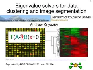
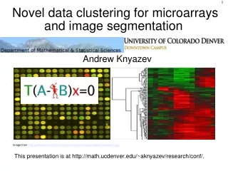
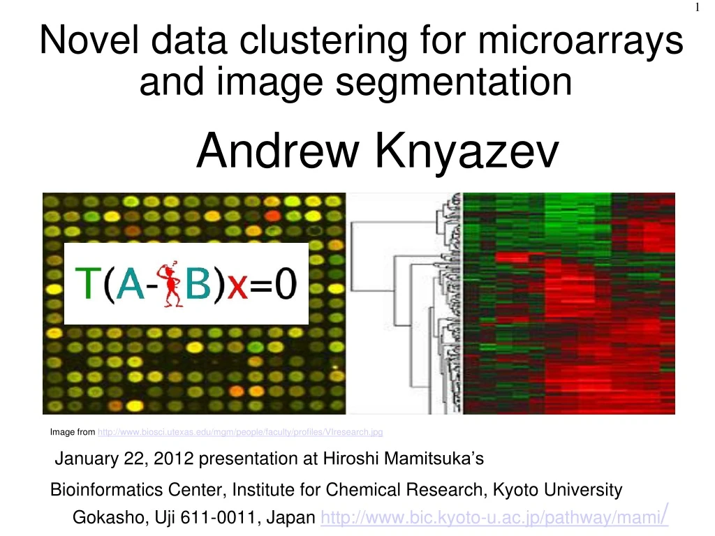
Novel data clustering for microarrays and image segmentation Andrew Knyazev Image from http://www.biosci.utexas.edu/mgm/people/faculty/profiles/VIresearch.jpg January 22, 2012 presentation at Hiroshi Mamitsuka’s Bioinformatics Center, Institute for Chemical Research, Kyoto University Gokasho, Uji 611-0011, Japan http://www.bic.kyoto-u.ac.jp/pathway/mami/
Abstract: We develop novel algorithms and software on parallel computers for data clustering of large datasets. We are interested in applying our approach, e.g., for analysis of large datasets of microarrays or tiling arrays in molecular biology and for segmentation of high resolution images.
Contents • Microarrays---a massively parallel experiment • Clustering: why? • Clustering: how? • Spectral clustering • Connection to image segmentation • Eigensolvers for spectral clustering
Microarrays-massivelyparallel experiment 1/5 Affymetrix GeneChip DNA Microarrays Image Courtesy: Affymetrix
Microarrays-massively parallel experiment 2/5 • GeneChip: oligonucleotide sequences are photo-lithographed on a quartz wafer in a pattern of ~10 micrometers dots. • Oligonucleotide sequences (oligos) probes: 25 nucleotide chains for selected parts of a gene complementary to mRNA. • GeneChips are manufactured to include all currently known and predicted genes of a particular organism, e.g., H. sapience. The information about physical locations of oligo probes for each gene on the chip is contained in the *.cdf file. • A sample of mRNA extracted from cells of an organism after pre-processing is hybridized with GeneChip giving PM and MM values which characterize genes expressions in the cells. For every gene there are 11-20(depending on chip design) of different oligo probes called perfect matches (PM). In addition, there are mismatch oligos (MM) corresponding to each of the PMs that differ in the middle base pair.
Microarrays-massively parallel experiment 3/5 • Labelled cRNA targets derived from the mRNA of an experimental sample are hybridized to oligo probes. • During hybridization, complementary nucleotides line up and bind together via hydrogen bonds in the same way as two strands of DNA bound together. • The chip is then scanned with a laser giving the amount of each mRNA species represented. • Image Courtesy: cnx.org
Microarrays-massively parallel experiment 4/5 • A pool of mRNA is extracted from the cells of an organism and converted to a Biotin labelled strand (cRNA) that binds to the oligo probes on the GeneChip during hybridization. • The higher the concentration of a particular mRNA in the testing pool---the greater the hybridization level of the PM probes and thus the amount of the hybridized material on the processed GeneChip. • Then a fluorescent stain is applied that binds to the Biotin and the GeneChip is processed through a scanner that illuminates each dot of the GeneChip with a laser, causing dots to fluoresce. • The image data of the scanned probe array is stored in a *.dat file. The Affymetrix GCOS software processes the *.dat file and generates a *.cel file, containing all numerical data of the GeneChip experiment, e.g., probe locations and PM and MM intensities. The processing involves computing a square grid locating the dots for probes, intensity normalization, using internal controls, and detecting the outliers. • More sophisticated *.dat-->*.cel algorithms, e.g., taking into account the cRNA saturation, are being developed elsewhere.
Microarrays-massively parallel experiment 5/5 • The PM and MM values are not normally used directly for high-level statistical analysis, instead they are first converted into the gene expression values, which involves: • Detecting unreliable data by comparing PM and MM • Adjustment for background and noise • Calculating the single array gene expression intensities, basically by averaging adjusted PM values for each probe set • Alternatively, the Comparison Analysis (Experiment versus Baseline arrays) detects and quantifies changes in gene expressions between two arrays, applying normalization of data and using the Signal Log Ratio algorithms. • Either way, the absolute or comparison gene expression values are stored in a *.chp file, which serves as the input for high-level statistical analysis. Typically, multiple GeneChip tests are performed giving multiple *.chp files with gene expression values.
Clustering: why? • When conducting microarray experiments there are multiple microarrays involved typically: • Studying a process over time,e.g., to measure the response to a drug or food. • Looking for differences between states, e.g., normal cells versus cancer cells. • A typical goal is Finding Gene Networks, i.e., groups of genes that change expression inter-dependently across samples. Having a significantly large number of microarrays, we want to reverse engineer the regulatory network that controls gene expressions. We need computer clustering on the microarray data to select a small (ideally) number of co-expressed genes of a gene network. Separate experiments using gene knockout on the selected genes can then be performed to confirm the discovered regulatory network biologically.
Clustering: how? The overview There is no good widely accepted definition of clustering. The traditional graph-theoretical definition is combinatorial in nature and computationally infeasible. Heuristics rule! Good open source software, e.g., METIS and CLUTO. Clustering can be performed hierarchically by agglomeration (bottom-up) and by division (top-down). Agglomeration clustering example
Clustering: how? Co-clustering Two-way clustering, co-clustering or bi-clustering are clustering methods where not only the objects are clustered but also the features of the objects, i.e., if the data is represented in a data matrix, the rows and columns are clustered simultaneously! Image courtesy http://www.gg.caltech.edu/~zhukov/research/spectral_clustering/spectral_clustering.htm
Clustering: how? Algorithms Partitioning means determining clusters. Partitioning can be used recursively for hierarchical division. Many partitioning methods are known. Here we cover: • Spectral partitioning using Fiedler vectors = Principal Components Analysis (PCA) PCA/spectral partitioning is known to produce high quality clusters, but is considered to be expensive as solution of large-scale eigenproblems is required. Our expertise in eigensolvers comes to the rescue!
Eigenproblems in mechanical vibrations Free transversal vibration without damping of the mass-spring system is described by the ODE system Standing wave assumption leads to the eigenproblem Component xi describes the up-down movement of mass i. Images courtesy http://www.gps.caltech.edu/~edwin/MoleculeHTML/AuCl4_html/AuCl4_page.html
Spectral clustering in mechanics The main idea comes from mechanical vibrations and is intuitive: in the spring-mass system the masses which are tightly connected will have the tendency to move together synchronically in low-frequency free vibrations. Analysing the signs of the components corresponding to different masses of the low-frequency vibration modes of the system allows us to determine the clusters of the masses! A 4-degree-of-freedom system has 4 modes of vibration and 4 natural frequencies: partition into 2 clusters using the second eigenvector: Images Courtesy: Russell, Ketteriung U.
Spectral clustering for simple graphs Undirected graphs with no self-loops and no more than one edge between any two different vertices • A = symmetric adjacency matrix • D = diagonal degree matrix • Laplacian matrix L = D – A L=K describes transversal vibrations of the spring-mass system (as well as Kirchhoff's law for electrical circuits of resistors)
Spectral clustering for simple graphs The Laplacian matrix L is symmetric with the zero smallest eigenvalue and constant eigenvector (free boundary). The second eigenvector, called the Fiedler vector, describes the partitioning. • The Fiedler eigenvector gives bi-partitioning by separating the positive and negative components only • By running the K-means on the Fiedler eigenvector one could find more then 2 partitions if the vector is close to piecewise-constant after reordering • The same idea for more eigenvectors of Lx=λx Example Courtesy: Blelloch CMU 1 2 5 3 www.cs.cas.cz/fiedler80/ 4 Rows sum to zero
PCA clustering for simple graphs • Fiedler vector is an eigenvector of Lx=λx, in the spring-mass system this corresponds to the stiffness matrix K=L and to the mass matrix M=I (identity) • Should not the masses with a larger adjacency degree be heavier? Let us take the mass matrix M=D -the degree matrix • So-called N-cut smallest eigenvectors of Lx=λDx are the largest for Ax=µDx with µ=1-λ since L=D-A • PCA for D-1A computes the largest eigenvectors, which then can be used for clustering by the K-means • D-1A is row-stochastic and describes the Markov random walk probabilities on the simple graph
Spectral clustering for image segmentation Image pixels serve as graph vertices. In 2D, we generate a sparse Laplacian, by comparing neighboring only 5 or 9 pixels when calculating the weights for the graph edges by comparing pixel colors. We follow the same basic procedure in 3D, only changing the 2D grid into 3D grid. Any grid can be used, as well as superpixels.
Examples: 2D image segmentation Image pixels serve as graph vertices. Weighted graph edges are computed by comparing pixel colours. Here is an example displaying 4 Fiedler vectors of a 2D image: We generate a sparse Laplacian, by comparing neighboring pixels here when computing the weights for the edges. Genes correspond to vertices in microarrays, but we have to compare all genes, possibly getting a Laplacian with a large fill-in.
3D vs. frame-by-frame 2D image segmentation The first image was taken from the 3D algorithm run over the entire ~10 frame animation, whereas the second one was taken from the 2D algorithm run on a single frame, 200x300
Eigensolvers for spectral clustering • Our BLOPEX-LOBPCG software has proved to be efficient for large-scale eigenproblems for Laplacians from PDE's and for image segmentation using multiscale preconditioning of hypre • The LOBPCG for massively parallel computers is available in our Block Locally Optimal Preconditioned Eigenvalue Xolvers (BLOPEX) package • BLOPEX is built-in in http://www.llnl.gov/CASC/hypre and available in http://www.grycap.upv.es/slepc/ • On BlueGene/L 1024 CPU the Fiedler vector of a 24 megapixel image takes seconds (including the hypre algebraic multigrid setup) to compute
Conclusions • LOBPCG is extremely efficient for 2D and 3D image segmentation • Using LOBPCG for DNA microarrays can be made more efficient by data graph sparsification