Download
1 / 1
10 likes | 154 Vues
Tomohito Yamada (tomohito@iis.u-tokyo.ac.jp). Tomohito YAMADA 1 ) , Shinjiro KANAE 2 ) , Taikan OKI 1 ) , and Randal D. KOSTER 3 ) 1) Institute of Industrial Science, The University of Tokyo 2) Research Institute for Humanity and Nature 3) NASA Goddard Space Flight Center.

E N D
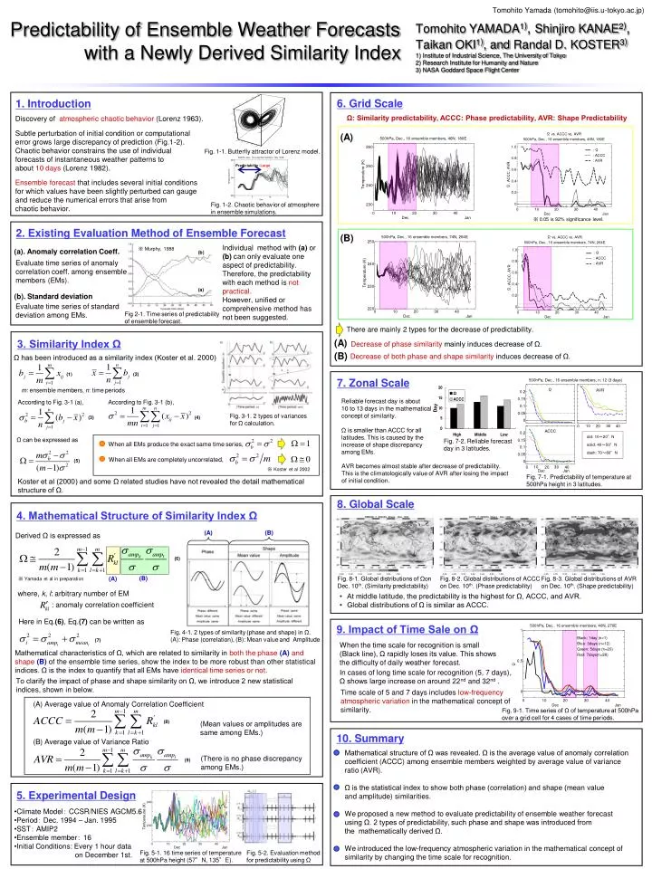
Tomohito Yamada (tomohito@iis.u-tokyo.ac.jp) Tomohito YAMADA1), Shinjiro KANAE2), Taikan OKI1), andRandal D. KOSTER3)1) Institute of Industrial Science, The University of Tokyo2) Research Institute for Humanity and Nature3) NASA Goddard Space Flight Center Predictability of Ensemble Weather Forecasts with a Newly Derived Similarity Index 6. Grid Scale 1. Introduction Ω: Similarity predictability, ACCC: Phase predictability, AVR: Shape Predictability Discovery of atmospheric chaotic behavior (Lorenz 1963). Subtle perturbation of initial condition or computational error grows large discrepancy of prediction (Fig.1-2). Chaotic behavior constrains the use of individual forecasts of instantaneous weather patterns to about 10 days (Lorenz 1982). Ensemble forecast that includes several initial conditions for which values have been slightly perturbed can gauge and reduce the numerical errors that arise from chaotic behavior. (A) Fig. 1-1. Butterfly attractor of Lorenz model. Predictability:Large Fig. 1-2. Chaotic behavior of atmosphere in ensemble simulations. ※ 0.05 is 92% significance level. 2. Existing Evaluation Method of Ensemble Forecast (B) Individual method with (a) or (b) can only evaluate one aspect of predictability. Therefore, the predictability with each method is not practical. However, unified or comprehensive method has not been suggested. ※ Murphy, 1988 (a). Anomaly correlation Coeff. (b). Evaluate time series of anomalycorrelation coeff. among ensemblemembers (EMs). (a) (b). Standard deviation Evaluate time series of standarddeviation among EMs. Fig 2-1. Time series of predictability of ensemble forecast. There are mainly 2 types for the decrease of predictability. (A) Decrease of phase similarity mainly induces decrease of Ω. 3. Similarity Index Ω (B) Decrease of both phase and shape similarity induces decrease of Ω. Ω has been introduced as a similarity index (Koster et al. 2000) (1) (2) 7. Zonal Scale m: ensemble members, n: time periods Reliable forecast day is about10 to 13 days in the mathematicalconcept of similarity. Ω is smaller than ACCC for all latitudes. This is caused by the increase of shape discrepancy among EMs. According to Fig. 3-1 (a), According to Fig. 3-1 (b), Day (3) (4) Fig. 3-1. 2 types of variances for Ω calculation. Ω can be expressed as Fig. 7-2. Reliable forecast day in 3 latitudes. When all EMs produce the exact same time series, When all EMs are completely uncorrelated, (5) AVR becomes almost stable after decrease of predictability. This is the climatologically value of AVR after losing the impact of initial condition. ※ Koster et al 2002 Fig. 7-1. Predictability of temperature at500hPa height in 3 latitudes. Koster et al (2000) and some Ω related studies have not revealed the detail mathematical structure of Ω. 8. Global Scale 4. Mathematical Structure of Similarity Index Ω (A) (B) Derived Ω is expressed as (6) (B) (A) Fig. 8-1. Global distributions of Ωon Dec. 10th. (Similarity predictability) Fig. 8-2. Global distributions of ACCCon Dec. 10th. (Phase predictability) Fig. 8-3. Global distributions of AVRon Dec. 10th. (Shape predictability) ※ Yamada et al in preparation where, k, l: arbitrary number of EM • At middle latitude, the predictability is the highest for Ω, ACCC, and AVR. • Global distributions of Ω is similar as ACCC. : anomaly correlation coefficient Here in Eq.(6), Eq.(7) can be written as 9. Impact of Time Sale on Ω Fig. 4-1. 2 types of similarity (phase and shape) in Ω.(A): Phase (correlation), (B): Mean value and Amplitude (7) When the time scale for recognition is small (Black line), Ω rapidly loses its value. This shows the difficulty of daily weather forecast. Mathematical characteristics of Ω, which are related to similarity in both the phase (A) and shape (B) of the ensemble time series, show the index to be more robust than other statistical indices. Ω is the index to quantify that all EMs have identical time series or not. In cases of long time scale for recognition (5, 7 days),Ω shows large increase on around 22nd and 32nd . To clarify the impact of phase and shape similarity on Ω, we introduce 2 new statistical indices, shown in below. Time scale of 5 and 7 days includes low-frequencyatmospheric variation in the mathematical concept ofsimilarity. (A) Average value of Anomaly Correlation Coefficient Fig. 9-1. Time series of Ω of temperature at 500hPaover a grid cell for 4 cases of time periods. (8) (Mean values or amplitudes aresame among EMs.) 10. Summary (B) Average value of Variance Ratio Mathematical structure of Ω was revealed. Ω is the average value of anomaly correlation coefficient (ACCC) among ensemble members weighted by average value of variance ratio (AVR). Ω is the statistical index to show both phase (correlation) and shape (mean value and amplitude) similarities. We proposed a new method to evaluate predictability of ensemble weather forecast using Ω. 2 types of predictability, such phase and shape was introduced from the mathematically derived Ω. We introduced the low-frequency atmospheric variation in the mathematical concept of similarity by changing the time scale for recognition. (There is no phase discrepancyamong EMs.) (9) 5. Experimental Design • Climate Model: CCSR/NIES AGCM5.6 • Period: Dec. 1994 – Jan. 1995 • SST: AMIP2 • Ensemble member: 16 • Initial Conditions: Every 1 hour data on December 1st. Fig. 5-1. 16 time series of temperatureat 500hPa height (57°N, 135°E). Fig. 5-2. Evaluation methodfor predictability using Ω