Download
1 / 78
790 likes | 1.06k Vues
Comparison of land surface models. CLIM 714 Randy Koster Paul Dirmeyer. GSWP. LAND SURFACE MODEL INTERCOMPARISONS. In recognition of the importance of land surface processes in the climate system, the international community developed various programs to characterize and

E N D
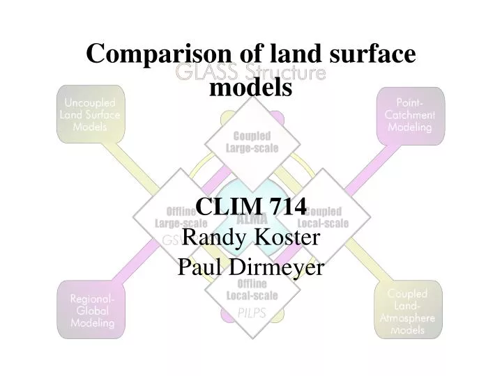
Comparison of land surface models CLIM 714 Randy Koster Paul Dirmeyer
GSWP LAND SURFACE MODEL INTERCOMPARISONS In recognition of the importance of land surface processes in the climate system, the international community developed various programs to characterize and compare land surface model behavior. Recently, these crystallized into a single encompassing structure: GLASS (Global Land-Atmosphere System Study) GCM inter-comparisons Global gridded model analyses Single column model analyses LoCo Land-surface model intercom-parisons (in situ)
Offline local scale PILPS PIs: Ann Henderson-Sellers, Andy Pitman Project for the Intercomparison of Land-Surface Parameterization Schemes (http://cic.mq.edu.au/pilps-rice) Text from a recent PILPS report: • PILPS is a community-driven initiative which provides opportunities to compare land-surface • schemes’ performance against others (past and present). Within this framework, PILPS serves • the international modelling community in two different and complementary ways: • a) by providing open, quality controlled intercomparison opportunities as international • benchmarks against which new and revised LSS can be validated; and • b) by providing the tools and intercomparison frameworks by means of which the behaviour • of LSS can be more fully understood. • The first of these, open to all who wish to participate, demands high quality observational data, • careful experimental design and agreed quality control procedures. The second involves a smaller • group of researchers and land-surface schemes with the specific goal of enhanced understanding. • The two questions being posed by these two complementary activities of PILPS are: • a) does your scheme perform well enough to be part of international modelling and prediction • efforts? • b) is it understood why your scheme performs the way it does?
PILPS has four levels of experimentation... Updates to table: PILPS2e was instead a study of land surface behavior in high northern latitudes (Torne-Kalix river basin in Sweden). PILPS - San Pedro was added: a study focusing on an arid regions. PILPS is also doing an intercomparison study focusing on carbon assimilation. A new study, just starting up, focuses on land effects on water isotope distributions.
PILPS 2e: Simulation of Arctic hydrology Torne-Kalix River Basin, Sweden Results show, e.g., a strong sensitivity of annual runoff to aerodynamic resistance formulation and its associated impact on snow sublimation.
PILPS San Pedro: An emphasis on parameter calibration/optimization
Unquantitative (first-order) characterization of the climates of PILPS studies (Don’t take the relative positions of the experiments here too seriously!) HOT San Pedro 1a Amazon (idealized) 2c Red-Arkansas 2b HAPEX- Mobilhy 2a Cabauw 2e Torne- Kalix 2d Valdai COLD WET DRY
The different PILPS studies generally had different foci: HOT Parameter calibration or optimization San Pedro 1a Amazon (idealized) 2c Red-Arkansas 2b HAPEX- Mobilhy 2a Cabauw Distributed studies Snowpack and other cold season processes 2e Torne- Kalix 2d Valdai COLD WET DRY
PILPS 3: Analyses of LSS behavior with AGCMs SiBlings Sfc. Energy Balances normalised by ensemble of 3 re-analyses – 3 clusters SiBlings Buckets Scaled sensible heat W m-2 SiBlings Buckets Buckets Scaled latent heat W m-2 Slide courtesy of Ann Henderson-Sellers
SnowMIP (Snow Model Intercomparison Project)(E. Martin and P. Etchevers at Meteo-France, CNRM) • Models show a wide range in the evolution of season snow pack (forced by identical atmospheric conditions). Slide courtesy of Adam Schlosser
www.iges.org/gswp/ gswp@cola.iges.org Global Soil Wetness Project • Overview • The Global Soil Wetness Project (GSWP) is an ongoing modeling activity of the International Satellite Land-Surface Climatology Project (ISLSCP) and the Global Land-Atmosphere System Study (GLASS), both contributing projects of the Global Energy and Water Cycle Experiment (GEWEX). GSWP is charged with producing large-scale data sets of soil moisture, temperature, runoff, and surface fluxes by integrating one-way uncoupled land surface schemes (LSSs) using externally specified surface forcings and standardized soil and vegetation distributions. • Motivation • The motivation for GSWP stems from the paradox that soil wetness is an important component of the global energy and water balance, but it is unknown over most of the globe. Soil wetness is the reservoir for the land surface hydrologic cycle, it is a boundary condition for atmosphere, it controls the partitioning of land surface heat fluxes, affects the status of overlying vegetation, and modulates the thermal properties of the soil. Knowledge of the state of soil moisture is essential for climate predictability on seasonal-annual time scales. However, soil moisture is difficult to measure in situ, remote sensing techniques are only partially effective, and few long-term climatologies of any kind exist. The same problems exist for snow mass, soil heat content, and all of the vertical fluxes of water and heat between land and atmosphere. • Goals • Produce state-of-the-art global data sets of soil moisture, surface fluxes, and related hydrologic quantities. • Develop and test large-scale validation techniques over land. • Provide large-scale validation and quality check of the ISLSCP data sets. • Compare LSSs, and conduct sensitivity studies of specific parameterizations which should aid future model development.
Global Soil Wetness Project GSWP-1 Data Issues
GSWP anomalies Free Soil moisture Relaxed Soil moisture From Douville and Chauvin, Climate Dyn. 2000 Sensitivity of JJAS climate to soil moisture relaxation toward GSWP: impact on soil moisture (kg/m²)
Runoff and gauge density • Spread is widest when gauge density is low • Errors are generally negative (too little runoff) Courtesy Taikan Oki
Global Soil Wetness Project GSWP-1 Validation Issues
Global Soil Wetness Project GSWP-1 Model Sensitivity Studies I
Global Soil Wetness Project GSWP-1 Model Sensitivity Studies II
Global Soil Wetness Project http://www.cnrm.meteo.fr/mc2/projects/rhoneagg/ Rhône-AGG – A study of the effects of spatial aggregation • Contacts: Aaron Boone, Florence Habets & Joel Noilhan • Météo-France, CNRM, Toulouse, France • The Rhône-AGGregation (Rhône-AGG) project will examine how various LSSs are able to simulate the river discharge over several annual cycles when inserted into the Rhône modeling system, and to explore the impact of the various scaling or aggregation methods on the simulation of certain components of the hydrological cycle. • The Rhône basin size is on the order of that of a coarse-resolution Global atmospheric Climate Model (GCM), but the atmospheric forcing, the soil and vegetation parameters, and the observed river discharges are available at a significantly higher spatial resolution, on the order of 8 km. • The Rhône modeling system, which was developed in recent years by the French research community, is comprised of three distinct components: • A distributed hydrological model • An analysis system to determine the near-surface atmospheric forcing • A SVAT model interface Rhône Basin and examples of (clockwise from top) the 8km grid for meteorological forcing data, topography, surface and sub-surface hydrology, vegetation, and distribution of rain gauges (+) and meteorological stations (▲).
Global Soil Wetness Project http://www.cnrm.meteo.fr/mc2/projects/rhoneagg/ Rhône-AGG – Results I The MODCOU hydrologic scheme was used to route runoff for validation. LSSs showed a wide range of skill, particularly in terms of daily discharge in small basins, where schemes with sub-grid runoff formulations fared best.
Global Soil Wetness Project http://www.cnrm.meteo.fr/mc2/projects/rhoneagg/ Rhône-AGG – Results II Total runoff and ET were similar among LSSs, but partitioning between components varied greatly, leading to different equilibrium soil water states.
Global Soil Wetness Project http://www.cnrm.meteo.fr/mc2/projects/rhoneagg/ Rhône-AGG – Results III LSSs with more complex snow schemes generally performed better. Explicit multi-layer treatments of thermodynamic properties and ripening led to better simulations. The only scheme whose snow simulation did not degrade at lower resolutions was the scheme with sub-grid altitude banding (VIC).
nd Global Soil Wetness Project • This phase of the project will take advantage of: • The10-year ISLSCP Initiative 2 data set • The ALMA data standards developed in GLASS • The infrastructure developed in the pilot phase of GSWP • GSWP-2 represents an evolution in multi-model large-scale land-surface modeling with the following goals: • Produce state-of-the-art global data sets of soil moisture, surface fluxes, and related hydrologic quantities. • Develop and test in situ and remote sensing validation, calibration, and assimilation techniques over land. • Provide a large-scale validation and quality check of the ISLSCP data sets. • Compare LSSs, and conduct sensitivity analyses of specific parameterizations. www.iges.org/gswp/ gswp@cola.iges.org
Participants • Operational centers (COLA and IIS) • Land surface modelers (15 models so far) • Evaluation group • Remote sensing application group • End users (hydrologists, civil engineers, biogeochemists, ecologists, educators, etc.)
MODEL Institute Bucket University of Tokyo CLM-TOP University of Texas at Austin CBM/CHASM Macquarie University, Australia CLASS Meteorological Service of Canada CLM NASA GSFC/HSB COLA-SSiB COLA ECMWF ECMWF HY-SSiB NASA GSFC/CRB ISBA MétéoFrance/CNRM LAPUTA Meteorological Research Institute, Japan Meteorological Agency LaD USGS & NOAA/GFDL MATSIRO Frontier RSGC MECMWF KNMI (Dutch MetOffice), Netherlands Mosaic NASA GSFC/HSB MOSES-2 Met Office, UK NOAH NOAA NCEP/EMC NSIPP-Catchment NASA GSFC/NSIPP (GMAO) ORCHIDEE IPSL, France SiBUC Kyoto University Sland University of Maryland SPONSOR Institute of Geography, Russian Academy of Sciences SWAP Institute of Water Problems, Russian Academy of Sciences VIC Princeton & NASA GSFC/HSB VISA, CLM-Top University of Texas at Austin GSWP-2 Modeling Status Baseline Integration • Submitted • Imminent • Probably • Maybe • Bowed out Via LIS
GSWP-2 Models (as of March 2005) Vertical structure shows soil layers for water (W) and temperature (T), and the maximum number of snow layers (S). Soil data sets are either supplied by GSWP-2 (g) or the model’s default (d). For vegetation distributions, GSWP-2 supplied datasets include IGBP (i) and SiB (s) categories; Sland has dynamic vegetation. Two models have different time steps for energy (E) and soil (S).
Input Data Sets • Land surface parameters for participating LSSs will be specified from the ISLSCP Initiative II data set. • Near-surface meteorological data at 3-hour time steps will come from the NCEP/DOE and ERA40 reanalyses. ISLSCP Initiative II is producing 1° global grids of the reanalysis data. GSWP will produce “hybrid” forcing data, combining the reanalysis model products with mean gridded observational data (precipitation, downward radiation, and temperature). The hybrid data preserves the observed time means, but uses reanalysis to provide variability on shorter (diurnal-synoptic) timescales. The hybrid process as applied to reanalysis precipitation, where rainfall rates are scaled by the mean error of the reanalysis compared to gridded observed monthly means.
ISLSCP Initiative II • Objectives: • Revisit global change modeling data requirements and algorithm approaches. • Provide user services to target community. • Develop science driven, satellite-derived vegetation data sets for global change process studies. • Validate ISLSCP II data sets. • ISLSCP II expands upon the ISLSCP I collection: • Spatial resolution is 1/4, 1/2, and 1 degree. • Temporal resolution covers 10-year period from 1986 to 1995. • New data sets added (e.g. Carbon modeling data sets). • ISLSCP II provides a comprehensive collection of high priority global data sets in a consistent data format and Earth projection. • http://islscp2.sesda.com
Precipitation Topography Clear-Sky Albedo Cloud Amount II Soil Carbon LW Radiation Fossil Fuel Emissions Vegetation Biophysics (fPAR)
2002 1999 Data Workshops Synthesis Workshops Reqts Workshops Final Data Collection Uniform Grid Uniform Documentation • Science Questions • Analysis Framework • Data Requirements Identify Potential Data Providers Data Providers Generate Data Sets Users Data Review Validation Peer Review Information System Design Documentation ISLSCP Data Collection Development Science Working Group (Monthly Telecons)
Data Process and Types Parameter data (monthly, yearly, fixed) ISLSCP-II GDT 1.2 ALMA standard 360 x 180 gathered format 1 x 1 degree land compress vector ASCII 90o N ~ 60o S NetCDF
Fig. 5 Example station density, for 23 Jul 98, of daily total precipitation reports for retrospective (left) and realtime (right) NLDAS data streams. Courtesy Ken Mitchell
Annual Runoff Error by Latitude Figure 15 of Oki et al., 1999. Courtesy Taikan Oki
What’s ‘Gauge Correction’? 1. Precipitation gauge cannot catch 100% of particles under the strong wind condition. 2. Systematic error depends also on the gauge shape, attachment height (see Sevurk and Klemm, 1989), besides wind speed. 3. It becomes a big error especially in case of snowfall. Courtesy Taikan Oki
Sevurk and Klemm, 1989 There are many kinds of gauges in the World !! Courtesy Taikan Oki
Activities for ‘Gauge Correction’ Pioneers:Sevruk(Switzerland), Goodison(Canada), and D. Yang(Alaska) WMO Intercomparisons Project of Precipitation Gauges Instruments and observing methods report (Sevruk and Hamon,1984; Goodison et al., 1989) Correspondence with various gauges and a WMO standard gauge (DFIR) was investigated. Courtesy Taikan Oki
WMO Intercomparisons Project Standard Gauge (DFIR) Courtesy Taikan Oki
Gauge Catch Ratio Versus Wind Speed Courtesy Taikan Oki
Total Compensation Ratio 100 % Courtesy Taikan Oki
ALMA Categories of Model Output Variables • Time-mean (fluxes) • General energy balance components • General water balance components • Evapotranspiration components • Streamflow • Instantaneous • Surface state variables • Sub-surface state variables • Variables for validation with remote sensed data • Cold season processes Examples of data layers from the ISLSCP data project.
Multi-Model Analysis A major product of GSWP2 will be a multi-model land surface analysis for the ISLSCP II period. This will be a land surface analog to the atmospheric reanalyses. There will be a climatological annual cycle data set, and a larger data set for the entire series. Compiling the results of multiple LSSs to produce a single analysis will provide a model-independent result. Of particular value, uncertainty estimates can be put on all of the fields, based on inter-model spread. Additional uncertainties regarding forcing data can be quantified, based on the results of the sensitivity studies. Example of the multi-model mean (inset) and spread in evapotranspiration over North America during one decad from GSWP1. Over some regions the models are in good agreement (e.g., the mid-Atlantic coast), but in others (e.g., New England) the spread among models exceeds the mean of the models (color scale is the same for both plots).