Download
1 / 22
220 likes | 964 Vues
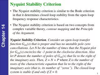
Nyquist (1). Hany Ferdinando Dept. of Electrical Engineering Petra Christian University. General Overview. Relation between Magnitude and Phase Angle Freq. response can be analyzed also via Polar Plot (the polar plot is also called as Nyquist plot) Advantages and disadvantages

E N D
Nyquist (1) Hany Ferdinando Dept. of Electrical Engineering Petra Christian University
General Overview • Relation between Magnitude and Phase Angle • Freq. response can be analyzed also via Polar Plot (the polar plot is also called as Nyquist plot) • Advantages and disadvantages • How to plot Nyquist using Matlab is discussed here Nyquist (1) - Hany Ferdinando
What? • Bode diagram uses two plots to show the frequency response of plants • Nyquist combines both plots into a single plot in polar coordinate as w is varied from 0 to ∞One must have knowledge in using complex number both in general notation and in phasor form Nyquist (1) - Hany Ferdinando
Polar Coordinate? • There are two parameters: • Radius, measured from the origin • Angle (from positive real axis) • Positive angle is counter clock wise • Negative angle is clock wise • For reference, students can study the general concept for algebra and geometry Nyquist (1) - Hany Ferdinando
Advantage and Disadvantage • Advantage: • It shows the frequency response characteristic of a system over the entire freq. range in a single plot • Disadvantage: • It does not clearly indicate the contribution of each individual factor of the open-loop transfer function Nyquist (1) - Hany Ferdinando
How to plot it? The idea is presented in: • Integral/derivative factor • First order factor • Quadratic factor Students have to exercise themselves how to plot the nyquist plot for other factors!!! Nyquist (1) - Hany Ferdinando
Derivative/integral factors (jw)±1 • Polar plot of (jw)-1 is negative imaginary axis • Polar plot of (jw) is positive imaginary axis Nyquist (1) - Hany Ferdinando
1st-order factors (1+jw)±1 • (1+jw)-1 • For w = 0 1 angle 0o • For w = 1/T 1/√2 angle -45o • For w = ∞ 0 angle -90o Nyquist (1) - Hany Ferdinando
1st-order factors (1+jw)±1 Nyquist (1) - Hany Ferdinando
1st-order factors (1+jw)±1 • (1+jw)-1 • For w = 0 1 angle 0o • For w = 1/T √2 angle 45o • For w = ∞ ∞ angle 90o Nyquist (1) - Hany Ferdinando
1st-order factors (1+jw)±1 Nyquist (1) - Hany Ferdinando
Quadratic Factor • [1+2z(jw/wn)+(jw/wn)2]-1 • For w0, G(jw) = 1 angle 0o • For w∞, G(jw) = 0 angle -180o Nyquist (1) - Hany Ferdinando
Quadratic Factor Nyquist (1) - Hany Ferdinando
Quadratic Factor • [1+2z(jw/wn)+(jw/wn)2] • For w0, G(jw) = 1 angle 0o • For w∞, G(jw) = ∞ angle 180o Nyquist (1) - Hany Ferdinando
Quadratic Factor Nyquist (1) - Hany Ferdinando
General Shapes of Polar Plot • Type 0 systems: the starting point (w=0) is finite on positive real axis. The tangent to polar plot at w=0 is perpendicular to the real axis. The terminal point (w=∞) is at the origin and the curve is tangent to one of the axes Nyquist (1) - Hany Ferdinando
General Shapes of Polar Plot • Type 1 systems: at w=0, the magnitude is infinity and phase angle is -90o. At w=∞, the magnitude is zero and the curve converges to the origin and is tangent to one of the axes Nyquist (1) - Hany Ferdinando
General Shapes of Polar Plot • Type 2 systems: at w=0, the magnitude is infinity and the phase angle is -180o. At w=∞ the magnitude becomes zero and the curve is tangent to one of the axes Nyquist (1) - Hany Ferdinando
w Type 2 ∞ w = 0 w ∞ ∞ 0 w w Type 0 w Type 1 0 Polar plot of type 0, 1 and 2 Nyquist (1) - Hany Ferdinando
n-m = 1 n-m = 1 n-m = 1 Polar Plot of high freq. range Nyquist (1) - Hany Ferdinando
Nyquist in Matlab • Use [re,im,w]=nyquist(sys) • ‘sys’ may be filled with (num,den) or transfer function or (A,B,C,D) in state space • In Nyquist, it is important to see the direction of the curve Nyquist (1) - Hany Ferdinando
Next… The Nyquist plot is already discussed, the subjects are to plot several general equation in Nyquist and how to use Matlab to plot nyquist. The next class is Nyquist stability criterion and phase-gain margin. Students have to prepare themselves for this topic. Nyquist (1) - Hany Ferdinando