Download
1 / 5

E N D
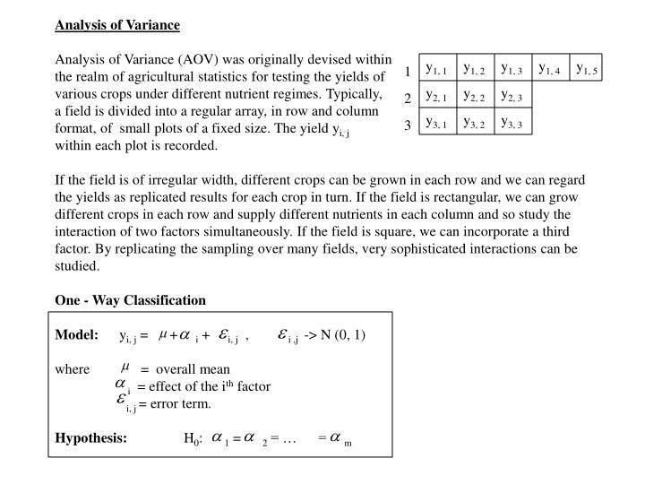
Analysis of VarianceAnalysis of Variance (AOV) was originally devised within the realm of agricultural statistics for testing the yields of various crops under different nutrient regimes. Typically, a field is divided into a regular array, in row and column format, of small plots of a fixed size. The yield yi, jwithin each plot is recorded. If the field is of irregular width, different crops can be grown in each row and we can regard the yields as replicated results for each crop in turn. If the field is rectangular, we can grow different crops in each row and supply different nutrients in each column and so study the interaction of two factors simultaneously. If the field is square, we can incorporate a third factor. By replicating the sampling over many fields, very sophisticated interactions can be studied.One - Way ClassificationModel: yi, j = + i + i, j , i ,j -> N (0, 1)where = overall mean i = effect of the ith factor i, j = error term.Hypothesis: H0: 1 = 2 = … = m y1, 1 y1, 2 y1, 3 y1, 4 y1, 5 1 y2, 1 y2, 2 y2, 3 2 y3, 1 y3, 2 y3, 3 3
Totals MeansFactor (1) y1, 1 y1, 2 y1, 3 y1, n1 T1 = y1, j y1. = T1 / n1 (2) y2, 1 y2,, 2 y2, 3 y1, n2 T2 = y2, j y2. = T2 / n2 (m) ym, 1 ym, 2 ym, 3 ym, nm Tm = ym, j ym. = Tm / nmOverall mean y = yi, j / n, where n = niDecomposition of Sums of Squares: (yi, j - y )2 = ni (yi . - y )2 + (yi, j - yi. )2 Total Variation (Q) = Between Factors (Q1) + Residual Variation (QE )Under H0: Q / (n-1) -> 2n - 1, Q1 / (m - 1) -> 2m - 1, QE / (n - m) -> 2n - m Q1 / ( m - 1 ) -> Fm - 1, n - m QE / ( n - m ) AOV Table:Variation D.F. Sums of Squares Mean Squares F Between m -1 Q1= ni(yi. - y )2 MS1 = Q1/(m - 1) MS1/ MSE Residual n - m QE= (yi, j - yi .)2 MSE = QE/(n - m) Total n -1 Q= (yi, j. - y )2 Q/( n - 1)
Two - Way Classification Factor I MeansFactor II y1, 1 y1, 2 y1, 3 y1, n y1. ym, 1 ym, 2 ym, 3 ym, n ym . Means y. 1 y. 2 y. 3 y . n yDecomposition of Sums of Squares: (yi, j - y )2 = n (yi . - y )2 + m (y. j - y )2 + (yi, j - yi . - y. j + y)2 Total Between Between Residual Variation Rows Columns VariationModel: yi, j = + i + j + i, j , i, j -> n ( 0, 1)H0: All i are equal and all j are equalAOV Table:Variation D.F. Sums of Squares Mean Squares F Between m -1 Q1= n (yi. - y )2 MS1 = Q1/(m - 1) MS1/ MSE Rows Between n -1 Q2= m (y.j - y )2 MS2 = Q2/(n - 1) MS2/ MSE Columns Residual (m-1)(n-1) QE= (yi, j - yi . - y. j + y)2 MSE = QE/(m-1)(n-1) Total mn -1 Q= (yi, j. - y )2 Q/( mn - 1)
Two - Way AOV [Example]Factor I 1 2 3 4 5 Totals Means Variation d.f. S.S. FFactor II 1 20 18 21 23 20 102 20.4 Rows 3 76.95 18.86** 2 19 18 17 18 18 90 18.0 Columns 4 8.50 1.57 3 23 21 22 23 20 109 21.8 Residual 12 16.30 4 17 16 18 16 17 84 16.8Totals 79 73 78 80 75 385 Total 19 101.75Means 19.75 18.25 19.50 20.00 18.75 19.25Note that many statistical packages, such as SPSS, are designed for analysing data that is recorded with variables values in columns and individual observations in the rows.Thus the AOV data above would be written as a set of columns or rows, based on the concepts shown:Variable 20 18 21 23 20 19 18 17 18 18 23 21 22 23 20 17 16 18 16 17Factor 1 1 2 3 4 5 1 2 3 4 5 1 2 3 4 5 1 2 3 4 5Factor 2 1 1 1 1 1 2 2 2 2 2 3 3 3 3 3 4 4 4 4 4 Normal Regression Model ( p independent variables) - AOVModel: y = 0 + i xi+ , -> n (0, s) Source d.f. S.S. M.S. FRegression p SSR MSR MSR/MSESSR = ( yi - y ) 2Error n-p-1 SSE MSE -SSE = ( yi - yi ) 2 SST = ( yj - y ) 2 Total n -1 SST - - Value of
Latin SquaresWe can incorporate a third source of variation in our A B C Dmodels by the use of latin squares. A latin square is a B D A Cdesign with exactly one instance of each “letter” in C A D Beach row and column. D C B AModel: yi, j = + i + j + l + i, j , i, j -> n ( 0, 1) Latin Square Component Column Effects Row EffectsDecomposition of Sums of Squares (and degrees of freedom) : (yi, j - y )2 = n (yi . - y )2 + n (y. j - y )2 + n (y. l - y )2 + (yi, j - yi . - y. j - yl + 2 y)2 Total Between Between Latin Square Residual Variation Rows Columns Variation Variation (n2 - 1) (n - 1) (n -1) (n - 1) (n - 1) (n - 2)H0: All i are equal, all i are equal and all i are equal.Experimental design is used heavily in management, educational and sociological applications. Its popularity is based on the fact that the underlying normality conditions are easy to justify, the concepts in the model are easy to understand and reliable software is available.