Download

1 / 29
300 likes | 396 Vues
DSP Pulse Detection System. Patrick Auchter Mark Paul. Project Goals. Detection of pulses in a low signal to noise ratio environment Requires a fast algorithm Rejection of noise spikes Less than 25% of identifications are false identifications Output the strength and frequency of pulse.

E N D
DSP Pulse Detection System Patrick Auchter Mark Paul
Project Goals • Detection of pulses in a low signal to noise ratio environment • Requires a fast algorithm • Rejection of noise spikes • Less than 25% of identifications are false identifications • Output the strength and frequency of pulse
System Overview • DSP samples at 44.1 kHz • 64 samples are collected every 1.45 ms • Input levels are -1 to 1 Volt • The processor is 80 MHz • Compiled code is loaded into the DSP through a parallel port using Code Composer Studio • The serial port is used to output binary data such as the pulse magnitude
Two-for-One FFT • A complex FFT is performed to take the FFT of two real sequences at once • The two output sequences are separated through the following equations
Assembly Buffer Setup 0 1 2 3 4 5 1020 1021 1022 1023 ↕ • The formulas for separating X(f) and Y(f) are
FFT Routine • First the input data is bit-reversed • Then a Radix-2 FFT is performed 000 → 000 001 → 100 010 → 010 011 → 110 100 → 001 101 → 101 110 → 011 111 → 111
Applying FFTs to Input Data • The DSP collects 64 new input samples every time the Two-for-One FFT is performed • The two buffers of FFT data are separated by 32 samples x 1 y x 2 y
Cost of the FFT • An N-point FFT costs N*log2(N) multiply-accumulates • After performing the two-for-one FFT, separating the two sequences requires 2*N additions • Using the two-for-one FFT saves us N*log2(N) multiply-accumulates, but adds 2*N additions • Calculating the magnitude of the frequency data requires 2*N multiplications and N additions
Detection Algorithm • A weighted average of the last 70 maximums in the frequency domain is calculated • Each maximum is multiplied by its corresponding weight and added to the total • The weighted average is the total divided by the sum of the weights • For a length 70 buffer, the sum of the weights is 42 • Computing the weighted average costs L multiply-accumulates, where L is the buffer length
Detection of Strong Pulses • The weighted average is used to determine if there is a pulse in the current window of FFT data • If the maximum is over 30 times the weighted average, it is definitely a pulse • Otherwise, we can check for a weak pulse
Detection of Weak Pulses • All of the FFT data over 3.4 times the weighted average is stored so that the width of the pulse can be determined • We check to make sure that the frequency difference of the points is less than or equal to 3 points or 258 Hz • We also check to make sure that the maximum in the current FFT data and the maximum in the previous FFT data are at the same frequency
Updating the Weighted Average • The following guidelines are used to determine when to update the weighted average • If the maximum is less than 3.4 times the weighted average, it is added to the maximum buffer and the weighted average is recalculated • Otherwise, the maximum is not added, since the maximum is either a noise spike or a pulse • Adding these maximums would undesirably increase the weighted average, making it more difficult to detect weak pulses
Challenges • Zero-padding and the two-for-one FFT • Designing a fast, efficient algorithm to process the data in real time • Testing all the data we collected and looking for abnormalities and weak pulses to test the system’s performance
Testing • Various signal-to-noise ratio signals were used to test and improve the system • Signals with odd noises were also tested to ensure that the noises did not cause false detections • We manipulated the following parameters to obtain the best results • FFT size • Length of the maximum buffer • Factors for determining strong and weak pulses • Length of the frequency window to analyze
Various SNR Signals 9.11 dB 3.09 dB -2.92 dB -6.44 dB
Effect of Decreasing Signal to Noise Ratio 9.11 dB 3.09 dB -2.92 dB -6.44 dB
Successes • The system consistently detects most of the audible pulses • When the pulse power is half the noise power, we detect the pulse 85 percent of the time • Less than 10% of the detections are noise • We do not use all of the clock cycles every pass, so additional processing of the data could be done if needed