Download
1 / 38
430 likes | 831 Vues
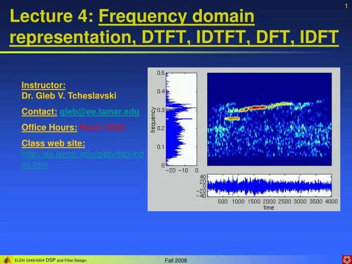
Lecture 4: Frequency domain representation, DTFT, IDTFT, DFT, IDFT. Instructor: Dr. Gleb V. Tcheslavski Contact: gleb@ee.lamar.edu Office Hours: Room 2030 Class web site: http://ee.lamar.edu/gleb/dsp/index.htm. Some history.

E N D
Lecture 4: Frequency domain representation, DTFT, IDTFT, DFT, IDFT Instructor: Dr. Gleb V. Tcheslavski Contact:gleb@ee.lamar.edu Office Hours: Room 2030 Class web site:http://ee.lamar.edu/gleb/dsp/index.htm
Some history Jean Baptiste Joseph Fourier was born in France in 1768. He attended the Ecole Royale Militaire and in 1790 became a teacher there. Fourier continued his studies at the Ecole Normale in Paris, having as his teachers Lagrange, Laplace, and Monge. Later on, he, together with Monge and Malus, joined Napoleon as scientific advisors to his expedition to Egypt where Fourier established the Cairo Institute. In 1822 Fourier has published his most famous work: The Analytical Theory of Heat. Fourier showed how the conduction of heat in solid bodies may be analyzed in terms of infinite mathematical series now called by his name, the Fourier series.
Frequency domain representation (4.3.1) frequency (4.3.2) complex exponent of 0 complex exponent of -0 A sinusoidal signal is represented by TWO complex exponents of opposite frequencies in the frequency domain.
Frequency domain representation (cont) (4.4.1) (4.4.2) Iff it exists! (4.4.3) (4.4.4) has a period of 2
Frequency domain representation (cont 2) For an arbitrary real LTI system: Symmetric with respect to Anti-symmetric with respect to
Frequency domain representation (cont 3) Combining(4.3.2)and(4.4.4) – back to our sinusoid! (4.6.1) (4.6.2) (4.6.3) (4.6.4) LTI filtering: from the input due to the input same as the input change due to the system phase change due to the system Via design, we manipulate H(ej), therefore, hn, and, finally, manipulate the coefficients in the Linear Constant Coefficient Difference Equation (LCCDE)
Frequency domain representation (cont 4) LCCDE: (4.7.1) (4.7.2) for large enough n: (4.7.3) (4.7.4)
Frequency domain representation (cont 5) for an LTI: (4.8.1) We don’t need systems of order higher than 2: can always make cascades. for a real, LTI, BIBO system: (4.8.2) effects of filtering We cannot observe ANY frequency components in the output that are not present in the input (in steady state). We may see less when
Frequency domain representation (cont 6) In continuous time: (4.9.1) signal noise const delay (4.9.2) We need a constant magnitude and linear phase for the frequencies of interest. LPF HPF BPF BSF Ideal filters: Ideal filters are non-realizable!
CTFT and ICTFT CTFT: (4.10.1) ICTFT: (4.10.2) Examples:
DTFT (4.11.1) if exists (4.11.2) (4.11.3) What’s about convergence??? 1. Absolute convergence: (4.11.4) (4.11.5)
DTFT (cont) Absolutely summable sequences always have finite energy. However, finite energy sequences are not necessary absolutely summable. must be 2. Mean-square convergence: (4.12.1) The total energy of the error must approach zero, not an error itself!
IDTFT (4.13.1) IDTFT: (4.13.2) Combining (4.11.1) and (4.12.2) (4.13.3) (4.13.4) shows where xn “lives” in the frequency domain.
Back to ideal filters (4.14.1) Ideal LPF: 1 Using IDTFT: 0 c 2 (4.14.2) • The response in (4.14.2) is not absolutely summable, therefore, the filter is not BIBO stable! • The response in (4.14.2) is not causal and is of an infinite length. As a result, the filter in (4.14.1) is not realizable. Similar derivations show that none of the ideal filters in slide 9 is realizable.
DTFT properties (4.15.1) (4.15.2) (4.15.3) (4.15.4) (4.15.5) (4.15.6) continuous, periodic functions (4.15.6)
DTFT examples (4.17.1) (4.17.2) (4.17.3) ½ of DC value of un (4.17.4) (4.17.5) (4.17.6)
DTFT examples (cont) We can re-work the Parseval’s theorem (4.15.6) as follows: (4.18.1) energy density (spectrum) Autocorrelation function: (4.18.2)
DTFT examples (cont 2) One obvious problem with DTFT is that we can never compute it since xn needs to be known everywhere! which is impossible! Therefore, DTFT is not practical to compute. Often, a finite dimension LTI system is described by LCCDE: (4.19.1) practical (finite dimensions) (4.19.2) Prediction of steady-state behavior of LCCDE
How to measure frequency response of an actual (unknown) filter? 1. Perform two I/O experiments: (4.20.1) (4.20.2) 2. Analyze these measurements and form: (4.20.3) (4.20.4) (4.20.5) That’s a good way to measure/estimate a frequency response for every .
DFT and IDFT Consider an N-sequence xn (at most N non-zero values for 0 n N-1) (4.21.1) uniformly spaced frequency samples DFT: (4.21.2) Finite sum! Therefore, it’s computable. (4.21.3) (4.21.1) can be rewritten as: (4.21.4) (4.21.5) Btw, DFT is a sampled version of DTFT.
DFT and IDFT (cont) Let us verify (4.21.5). We multiply both sides by (4.22.1) (4.22.2) (4.22.3) (4.22.4)
FFT (4.23.1) In the matrix form: (4.23.2) where: (4.23.3) (4.23.4) (4.23.5) (4.23.6) (4.23.7) This is actually FFT…
Relation between DTFT and DFT 1. Sampling of DTFT (4.24.1) (4.24.2) (4.24.3) yn is an infinite sum of shifted replicas of xn. Iff xn is a length M sequence (M N) than yn = xn. Otherwise, time-domain aliasing xncannot be recovered!
Relation between DTFT and DFT (cont) 2. DTFT from DFT by Interpolation Let xn be a length N sequence: Let us try to recover DTFT from DFT (its sampled version). (4.25.1) (4.25.2) (4.25.3) It’s possible to determine DTFT X(ej) from its uniformly sampled version uniquely!
Relation between DTFT and DFT (cont 2) 3. Numerical computation of DTFT from DFT Let xn is a length N sequence: defined by N uniformly spaced samples We wish to evaluate at more dense frequency scale. (4.26.1) Define: zero-padding (4.26.2) (4.26.3) No change in information, no change in DTFT… just a better “plot resolution”.
A note on WN (4.27.1) (4.27.2) WN is also called an Nth root of unity, since Im Im Re Re
DFT properties 1. Circular shift xn is a length N sequence defined for n = 0,1,…N-1. An arbitrary shift applied to xn will knock it out of the 0…N-1 range. Therefore, a circular shift that always keeps the shifted sequence in the range 0…N-1 is defined using a modulo operation: (4.28.1) (4.28.2)
DFT properties (cont) 2. Circular convolution A linear convolution for two length N sequences xn and gn has a length 2N-1: (4.29.1) A circular convolution is a length-N sequence defined as: (4.29.2) N N (4.29.3) Procedure: take two sequences of the same length (zero-pad if needed), DFT of them, multiply, IDFT: a circular convolution.
DFT properties (cont 2) Example: (4.30.1) Take N frequency samples of (4.30.1) and then IDFT: (4.30.2) aliased version of xn The results of circular convolution differ from the linear convolution “on the edges” – caused by aliasing. To avoid aliasing, we need to use zero-padding…
Linear filtering via DFT Often, we need to process long data sequences; therefore, the input must be segmented to fixed-size blocks prior LTI filtering. Successive blocks are processed one at a time and the output blocks are fitted together… We can do it by FFT: IFFT{FFT{x}FFT{h}}… Problem: DFT implies circular convolution – aliasing! (4.31.1) Assuming that hn is an M-sequence, we form an N-sequence (L - block length): (4.31.2) N >> M; L >> M; N = L + M - 1 and is a power of 2
Linear filtering via DFT (cont) Next, we compute N-point DFTs of xm,n and hn, and form (4.32.1) - no aliasing! Since each data block was terminated with M -1 zeros, the last M -1 samples from each block must be overlapped and added to first M – 1 samples of the succeeded block. An Overlap-Add method.
Linear filtering via DFT (cont 2) Alternatively: Each input data block contains M -1 samples from the previous block followed by L new data samples; multiply the N-DFT of the filter’s impulse response and the N-DFT of the input block, take IDFT. Keep only the last L data samples from each output block. The first block is padded by M-1 zeros. An Overlap-Save method.
DFT properties: General from Mitra’s book Btw, g[n] = gn
DFT properties: Symmetry from Mitra’s book xn is a real sequence
DFT properties: Symmetry (cont) from Mitra’s book xn is a complex sequence
N-point DFTs of 2 real sequences via a single N-point DFT Let gn and hn are two length N real sequences. Form xn = gn + jhn Xk (4.37.1) (4.37.2) (4.37.3) (4.37.4)