Download
1 / 34
350 likes | 508 Vues
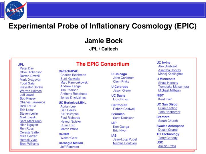
Experimental Probe of Inflationary Cosmology (EPIC). Jamie Bock JPL / Caltech. UC Irvine Alex Amblard Asantha Cooray Manoj Kaplinghat U Minnesota Shaul Hanany Tomotake Matsumura Michael Milligan NIST Kent Irwin UC San Diego Brian Keating Tom Renbarger Stanford Sarah Church

E N D
Experimental Probe of Inflationary Cosmology (EPIC) Jamie Bock JPL / Caltech UC Irvine Alex Amblard Asantha Cooray Manoj Kaplinghat U Minnesota Shaul Hanany Tomotake Matsumura Michael Milligan NIST Kent Irwin UC San Diego Brian Keating Tom Renbarger Stanford Sarah Church Swales Aerospace Dustin Crumb TC Technology Terry Cafferty USC Aluizio Prata The EPIC Consortium JPL Peter Day Clive Dickenson Darren Dowell Mark Dragovan Todd Gaier Krzysztof Gorski Warren Holmes Jeff Jewell Bob Kinsey Charles Lawrence Rick LeDuc Erik Leitch Steven Levin Mark Lysek Sara MacLellan Hien Nguyen Ron Ross Celeste Satter Mike Seiffert Hemali Vyas Brett Williams Caltech/IPAC Charles Beichman Sunil Golwala Marc Kamionkowski Andrew Lange Tim Pearson Anthony Readhead Jonas Zmuidzinas UC Berkeley/LBNL Adrian Lee Carl Heiles Bill Holzapfel Paul Richards Helmut Spieler Huan Tran Martin White Cardiff Walter Gear Carnegie Mellon Jeff Peterson U Chicago John Carlstrom Clem Pryke U Colorado Jason Glenn UC Davis Lloyd Knox Dartmouth Robert Caldwell Fermilab Scott Dodelson IAP Ken Ganga Eric Hivon IAS Jean-Loup Puget Nicolas Ponthieu
US Activities and Opportunities • NASA funded 3 mission studies for the Einstein “Inflation Probe” in 2003 • Envisioned as $350-$500M mission, launch 2010 & every 3 years • Since 2003 there have been some programmatic changes at NASA… • Oral reports were given at NASA HQ this month • Written reports are still being drafted • Task Force For CMB Research (Weiss Committee) in 2005 • Programmatic and technical roadmap to a 2018 launch for US agencies • Two mission options described • Sets mission guidelines: r = 0.01 is science goal • NRC panel to recommend first Beyond Einstein mission to NASA • First Beyond Einstein mission funding is to turn on 2008-9 • CMBPOL, Con-X, LISA, JDEM (aka SNAP), and Black Hole Finder • Recommendation based on “scientific merit and technical readiness” • NRC also to recommend areas for technology funding for next 4 BE missions • Three CMBPOL study teams will organize a single presentation to NRC • MIDEX call expected in October 2007 • Expected cap $220 - $260M including launch vehicle and 30 % cost reserve • Launch 2013 - 2015 • International participation in MIDEX’s limited in the past (~30 %) • Unknown if NASA would change the rules for this AO... probablyunlikely
Two Mission Scenarios for CMBPOL • Gravitational-Wave BB Polarization • Clear Justification for Space Mission • - Large angular scales required • Modest Mission Parameters • - Enough sensitivity to hit lensing limit • - Angular resolution to probe ℓ = 100 • - Broad frequency coverage • High-ℓ Science • Lensing BB signal • - How deeply can we remove lensing? • - Will foregrounds limit us first? • - How much more science do we get? • - Do we need to go to space for this? • EE power spectrum to cosmic variance • - Much will be done from the ground T Scalars Dust E r = 0.3 B Synch IGWs Cosmic Shear r = 0.01 B
EPIC is a Scan-Imaging Polarimeter Scan detectors across sky to build CMB map Simple technique. Established history in CMB. Scaling to higher sensitivity →Only need better arrays Adapt this technique for precision polarimetry Two mission concepts* Low Cost: High-TRL, low-resolution, sufficient capability Comprehensive Science: Larger aperture, new arrays *See Weiss Committee TFCR Report: astro-ph 0604101 Boomerang BICEP Planck Polarbear Maxipol QUaD EBEX Spider PLANNED FUTURE PAST ACTIVE
Optical Axis Spin Axis (~1 rpm) Orbit 55° Moon 45° Sun-Spacecraft Axis (~1 rph) Sun Earth SE L2 Why Space? - All-Sky Coverage - High Sensitivity - Systematic Error Control - Broad Frequency Coverage
Spin Axis (~1 rpm) 55˚ Optical Axis Precession (~1 rph) 45˚ Sun-Spacecraft Axis Downlink To Earth Scan Strategy Scan Coverage 1 minute 3 minutes 1 hour
Spin Axis (~1 rpm) 55˚ Optical Axis Precession (~1 rph) 45˚ Sun-Spacecraft Axis Downlink To Earth Scan Strategy 1 Day Maps Spatial Coverage Angular Uniformity More than half the sky in a single day!
Redundant & Uniform Scan Coverage N-hits (1-day) Angular Uniformity* (6-months) Planck WMAP EPIC 1 0 *<cos2b>2 + <sin 2b>2
EPIC Low Cost Mission Architecture Liquid Helium Cryostat (450 ℓ) 30/40 GHz 60 GHz 2 x 90 GHz 135 GHz 200/300 GHz Deployed Sunshield Six 30 cm Telescopes Commercial Spacecraft Solar Panels Absorbing Forebaffle 40 K Half-Wave Plate 2 K Refracting Optics 100 mK Focal Plane Array 100 K 155 K 295 K 8 m 3-Stage V-Groove Radiator Delta 2925H 3-m Toroidal-Beam Antenna
Comprehensive Science Mission Architecture 40 K Passively Cooled Mirrors 2.8 m Receiver & Lenses 85 K 155 K 293 K 3-Axis S/C Solar Panels Gimballed Antenna 3-Stage Sunshield Wrap-Rib Deployment LHe Dewar or Cryocooler 3-Stage V-Groove Atlas V 551 20 m
Sensitivity with Existing Detector Arrays EPIC Projected Bands and Sensitivities Absorbing Baffle (40 K) Half-Wave Plate (2 K) *Design Sensitivity †Goal Sensitivity 30 cm Aperture Stop (2 K) Note modest detector improvement over Planck due to relaxed time constant specification & 2 K optics Polyethylene Lenses (2 K) Planck Projected Sensitivities Telecentric Focus Focal Plane Bolometer Array (100 mK)
NTD Bolometers for Planck & Herschel 143 GHz Spider-web Bolometer Planck/HFI focal plane (52 bolometers) NTD Germanium SPIRELow-power JFETs Herschel/SPIRE Bolometer Array
Antenna-Coupled Bolometers for EPIC Measured Beam Patterns X-polarization Y-polarization 8 mm Measured Spectral Response High Optical Efficiency! Single Pixel – Dual Pol at 150 GHz (JPL/CIT) Advantages Small active volume.. 30 – 300 GHz operation Beam collimation…... Eliminates discrete feeds Reduced focal plane mass Intrinsic filters…….... No discrete components Kuo et al. SPIE 2006
Low-Cost Mission: High Technology Readiness New technologies bring enhanced capabilities… Antenna-Coupled TES / MKID detectors Higher sensitivity, less mass & power Continuously rotating waveplate Better beam control Continuous ADR Less mass, no interruptions …but we have the technology to do this mission today
TES Bolometer Arrays SQUID Multiplexing Advantages Multiplexing……. Larger array formats Higher sensitivity Fewer wires to 100 mK Low cryogenic power disp. Faster response... Useful for larger aperture Freq. Domain (UCB/LBNL) Time Domain (NIST) SCUBA2 Focal Plane (10,000 TES Bolometers) Antenna-Coupled TES Bolometers (UCB/LBNL)
Low-Cost Mission Focal Plane Options Input Assumptions Fractional bandwidth Dn/n = 30 % Optical efficiency h = 40 % Focal plane temperature = 100 mK Optics temperature = 2 K, with 10 % coupling Waveplate temperature = 20 K, with 2 % coupling Baffle at 40 K with 0.3 % coupling (measured) Psat/Q = 5 for TES bolometers G0 = 10 Q / T0 for NTD bolometers 1Sensitivity with 2 noise margin in a 1-year mission 2Calculated sensitivity in 2-year design life 3Two bolometers per focal plane pixel 4Sensitivity of one bolometer in a focal plane pixel 5Sensitiivity dT in a pixel qFWHM x qFWHM times qFWHM 6Sensitivity dT in a 120′ x 120′ pixel 7Combining all bands together
Systematic Error Mitigation Strategy * = Already demonstrated to EPIC requirement † = Proof of operation but needs improvement ‡ = Planned demonstration to EPIC requirement
Wide-Field Refracting Optics • Wide unaberrated FOV • Excellent main beams • Telecentric focus • Waveplate = first optic • Ultra-low sidelobes • Field tested in BICEP BICEP
Wide-Field Refracting Optics BICEP *Strehl ratio > 0.95
Polarization Systematics: Main Beams Main Beam Instrumental Polarization Effects • Calculation • Difference PSB beam pairs • Parameterize main beam effects • Convolve w/ scan pattern • Calculate resulting power spectrum • Caveats • Calculation is conservative → single pixel • We can always apply post facto correction • Waveplate eliminates these effects Differential FWHM Differential Gain, Rotation Differential Beam Offset Differential Ellipticity
Main Beam Properties at 135 GHz Performance at FOV Center *Goal: Suppress effect without correction below noise **Req’t: Suppress effect with correction below r = 0.01 †Calc: Worst performance over the FOV at 135 GHz ‡Meas: Median value measured in BICEP receiver PSF Performance at FOV Edge Difference Beam PSF Difference Beam
1e5 1e4 1e3 100 10 1 mK 100 30 10 3nK Far-Sidelobe Performance Sky at 100 GHz BICEP Measurements Sidelobe Map at 100 GHz ~ 20% polarized Levels below 3 nK for most of the sky!
EPIC WMAP-8 Planck Foregrounds - What We Know Today Input Sky Model Sensitivity per 14′ Pixel 75% of sky 75% of sky • 2. Multi-band Removal • Fit only synch & thermal dust • Fit components spectrally • Let indicies float spatially • 1. Input Sky Model • All components we • know about today 2% patch 2% patch Eriksen et al. 2006 Resulting Sensitivity After Subtraction • 3. Results • Removal gives a modest sensitivity loss • Better sensitivity → better subtraction (model is linear) • 4. Conclusion: FGs Look Manageable! • Preliminary. We might find a new component tomorrow • We don’t know where a linear model fails nKCMB in 2˚ pixels
Conclusions Exciting CMB science in the post-Planck era § Clear role for gravitational-wave polarization science in space § High-ℓ science compelling but need for space is less robust Imaging polarimeter approach § Technically and scientifically feasible § Simple technique, established history. §Simple scaling to higher sensitivity: improve the focal plane. § Design in extensive control of systematics from the beginning § Low-Cost option → meets Weiss Committee guidelines for GW science § Comprehensive Science option → more capable, more science, more $ Foregrounds § What we know today about polarized foreground shows they can be subtracted below r = 0.01 Technologies § We can build a very capable mission today with existing technology § New technologies will improve the mission & reduce technical risk