Download
1 / 41
410 likes | 611 Vues
Significance analysis of microarrays applied to the ionizing radiation response. Presented by Wenlei Liu Department of Health Evaluation Sciences September 19, 2004. Goal. Differential Analysis of Microarray data :

E N D
Significance analysis of microarrays applied to the ionizing radiation response Presented by Wenlei Liu Department of Health Evaluation Sciences September 19, 2004
Goal Differential Analysis of Microarray data : Individually identifying genes differentially expressed between two conditions
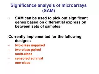
Problem • People usually use conventional t tests to test the null hypothesis of no difference in intensity across conditions for each gene. This will result in multiple testing problem. Normal assumption may be invalid. • Significance analysis of microarrays (SAM) identifies significantly differentially expressed genes using a permutation procedure.
Experiment Study the transcriptional response of lymphoblastoid cells to ionizing radiation (IR). Two cell lines (1 & 2) were used. Allow cell lines to grow in unirradiated state (U) or in an irradiated state (I) 4 hours after exposure to a modest dose of 5 Gy of ionizing radiation (IR). Divide RNA samples into two parts and performed two independent hybridizations, A and B. Eight chips– U1A, U1B, U2A, U2B, I1A, I1B, I2A, I2B.
Microarray hybridization • Each gene was represented by 20 oligonucleotide pairs. Each pair has an perfectly matched oligonucleotide and an oligonucleotide containing one base mismatch. Gene expression levels were calculated from differences in hybridization to the matched and mismatched probes by GENECHIP software.The expression levels could be negative.
Scale expression levels from two hybridizations • Generate a reference data set by averaging the expression of each gene over eight hybridizations. • Compare data for each hybridization with the reference data set in a cube root scatter plot. • Use a linear least-squares fit to the cube root scatter plot to calibrate each hybridization.
Methods • The “relative difference”
Permutation procedure • Use 36 permutations that are balanced for cell lines 1 and 2. • Rank the genes by their d(i) values. • Calculate dp(i) for each of the 36 permutations. • Compute the expected relative difference dE(i) , dE(i)= pdp (i) /36. • Compare the observed d(i) vs. the expected dE(i)
Example • Original Ranked
Identification of genes with significant changes in expression
False discovery rate (FDR) • Define the smallest positive d(i) and the largest negative d(i) among the significant genes to be the horizontal cutoffs. • In each permutation, count the number of genes that exceed the horizontal cutoffs. • The estimated number of falsely significant genes is the average of the number of falsely significant genes from all 36 permutations. • The estimated FDR equals the estimated number of falsely significant genes divided by the significant genes.
Comparison with other methods Compare SAM with Fold change method – gene (i) is significant if r(i) > R or < 1/R Pairwise fold change –compute pairwise fold change using four data sets in state U and state I. A gene is significant if 12 of 16 pairings satisfied the above criteria.
Validation • Randomly select genes from 46 significant genes identified by SAM (=1.2) and 57 significant genes identified by fold change method (at least 3.6 fold change) to perform Northern blot. • Little correlation with genes identified by the fold change method, but strong correlation with the genes identified by SAM.
Comparison of SAM to conventional methods for analyzing microarrays
Conclusion • SAM is more reliable than other methods. • SAM successfully decreases the false positive rate.
Diagnosis of multiple cancer types by shrunken centroids of gene expression
Problems • Cancers have many different types. For example, leukemia includes Acute myeloid leukemia (AML), Acute lymphocytic leukemia (ALL), Chronic myelogenous leukemia (CML) and Chronic lymphocytic leukemia (CLL). • Successful cancer treatment depends on an accurate and correct diagnosis. • Traditional cancer diagnosis examines the morphological appearance of stained tissue specimens in the light microscope. This method requires highly trained pathologists and it is subjective.
The impact Errors in the Biopsy Diagnosis of Cancer can lead to: • Unnecessary or incorrect cancer treatment (surgery, chemotherapy, radiation) with serious complications or long-term disability when a benign lesion is incorrectly diagnosed as malignant. • A missed opportunity to treat a curable cancer-- especially when an early malignant lesion is incorrectly diagnosed as non-cancerous or inadequately sampled. • Unnecessary and costly medical expenses. • Avoidable pain and suffering
Goal • Classify and predict cancer category of a sample based on its gene expression profile. • Microarray cancer classification could be objective and highly accurate. • Identify the smallest subset of genes from a large number of genes. Assign samples into distinct categories based on expression of the subset of genes.
Nearest-centroid classification Centroid – C(x) = k, where xij denotes the expression of genes i=1, 2, …, p and samples j=1, 2, ..n. k indexes the cancer classes.
Nearest shrunken centroid classification • Shrink the class centroids toward the overall centroids after standardizing by the within-class standard deviation for each gene.
Nearest shrunken centroid classification (cont’d) Shrink each dik towards zero, giving dik’ and new shrunken centroids
Nearest shrunken centroid classification (cont’d) • The shrinkage is down by soft thresholding: For example, For gene i, if dik’=0 for all k, then for all k. Gene i does not contribute to the nearest centroid computation. was chosen by cross-validation.
Discriminant functions For a test sample with expression levels The discriminant score for class k where k is the prior probability of class k and k=1. And Classification rule
Class probabilities • Use discriminant scores to construct estimates of class probabilities:
Samples Small round blue cell tumors (SRBCT) of childhood. • Tumors classified as Burkitt lymphoma (BL), Ewing sarcoma (EWS), neuroblastoma (NB), or rhabdomyosarcoma (RMS). • There were 63 training samples and 25 test samples. Five of the test samples were not SRBCT. 2308 genes were studied.
Choosing the amount of shrinkage • 10-fold cross validation – randomly divide the samples into 10 balanced equal-size groups. • Fit the modeling using 90% of the samples and then predict the class lables of the remaining 10% of the samples. • Repeat 10 times and compute misclassification error rate based on 10 repeats. 1 2 3 4 5 6 7 8 9 10 Train Train Train Train Train Train Train Train Train Test
Leukemia classification • Leukemia classified as ALL (acute lymphocytic leukemia) and AML (acute mylogenous leukemia). • 20 ALL samples and 14 AML samples. 7129 genes were studied using Affymetrix arrays.
Conclusion • Nearest shrunken centroids method was abele to assign SBRCTs to the correct class with 100% accuracy. • Nearest shrunken centroids method identify more known diagnostic SBRCT genes than other study. • Nearest shrunken centroids method classified leukemia samples with a lower error rate than other study and identify known diagnostic markers.
Software • http://www-stat.stanford.edu/~tibs/