Download

1 / 44
490 likes | 771 Vues
ANOVA. verginica. versicolor. setosa. The same slopes, but different intercepts. setosa. versicolor. verginica. factor (categoriacal) variable. dummy variables. for verginica. for versicolor. for setosa. setosa. versicolor. verginica. factor (categoriacal) variable.

E N D
verginica versicolor setosa The same slopes, but different intercepts
setosa versicolor verginica factor (categoriacal) variable dummy variables for verginica for versicolor for setosa
setosa versicolor verginica factor (categoriacal) variable dummy variables for verginica for versicolor for setosa
Equivalence of group means R adopts this convention. ANOVA : Analysis of Variances A statistical method for comparisons of (population) means of many groups. For comparison of two groups, t-test is applicable. ANOVA is a generalized method of t-test in this view. ANOVA does not aim to compare variances.
> is.factor(iris$Species) [1] TRUE > rout<- lm(Sepal.Length~Species,data=iris) > anova(rout) Analysis of Variance Table Response: Sepal.Length Df Sum Sq Mean Sq F value Pr(>F) Species 2 63.212 31.606 119.26 < 2.2e-16 *** Residuals 147 38.956 0.265 > summary(rout) Coefficients: Estimate Std. Error t value Pr(>|t|) (Intercept) 5.0060 0.0728 68.762 < 2e-16 *** Speciesversicolor 0.9300 0.1030 9.033 8.77e-16 *** Speciesvirginica 1.5820 0.1030 15.366 < 2e-16 *** Residual standard error: 0.5148 on 147 degrees of freedom Multiple R-squared: 0.6187, Adjusted R-squared: 0.6135 F-statistic: 119.3 on 2 and 147 DF, p-value: < 2.2e-16 This results support . That is, group means of sepal.length are not the same (at least one group has different group mean to the other two groups.
Comparison for the weights of tomato according to the treatment (trt). There are 3 treatment groups; water, nutrient, and nutrient with 2,4D component. The aim of this study is to see whether the nutrient and the 2,4D will increase (or decrease) the weight of tomato. Tomato data
> x<- c(1.5,1.9,1.3,1.5,2.4,1.5,1.5,1.2,1.2,2.1,2.9,1.6, + 1.9,1.6,0.8,1.15,0.9,1.6) > tx<- rep(c("water", "Nutrient", "Nutrient+24D"), c(6, 6, 6)) > ( tomato <- data.frame(weight=x, trt =tx ) ) > stripchart(weight~trt,pch=16, cex=1.4 ,col="red", data=tomato) > with(tomato, points(weight,trt, pch=16, cex=0.6 ,col="yellow")) Tomato data
> is.factor(tomato$trt) [1] TRUE > (sout1<- lm(weight~trt,data=tomato) ) Call: lm(formula = weight ~ trt, data = tomato) Coefficients: (Intercept) trtNutrient+24D trtwater 1.75000 -0.42500 -0.06667 > tomato$trt <- relevel(tomato$trt, ref="water") > (sout2<- lm(weight~trt,data=tomato) ) Call: lm(formula = weight ~ trt, data = tomato) Coefficients: (Intercept) trtNutrient trtNutrient+24D 1.68333 0.06667 -0.35833 > anova(sout1) Analysis of Variance Table Response: weight Df Sum Sq Mean Sq F value Pr(>F) trt 2 0.6269 0.31347 1.2019 0.328 Residuals 15 3.9121 0.26081 sout1 and sout2 are the same analysis, but use different base levels.
for nutrient+24D for nutrient for water
> summary(sout1) Call: lm(formula = weight ~ trt, data = tomato) Residuals: Min 1Q Median 3Q Max -0.5500 -0.3500 -0.1792 0.2750 1.1500 Coefficients: Estimate Std. Error t value Pr(>|t|) (Intercept) 1.75000 0.20849 8.394 4.74e-07 *** trtNutrient+24D -0.42500 0.29485 -1.441 0.170 trtwater -0.06667 0.29485 -0.226 0.824 > summary(sout2) Call: lm(formula = weight ~ trt, data = tomato) Coefficients: Estimate Std. Error t value Pr(>|t|) (Intercept) 1.68333 0.20849 8.074 7.69e-07 *** trtNutrient 0.06667 0.29485 0.226 0.824 trtNutrient+24D -0.35833 0.29485 -1.215 0.243 Residual standard error: 0.5107 on 15 degrees of freedom Multiple R-squared: 0.1381, Adjusted R-squared: 0.02321 F-statistic: 1.202 on 2 and 15 DF, p-value: 0.328 Everything is the same for sout1 and sout2 except the base levels. No sure evidence of and
> anova(sout2) Analysis of Variance Table Response: weight Df Sum Sq Mean Sq F value Pr(>F) trt 2 0.6269 0.31347 1.2019 0.328 Residuals 15 3.9121 0.26081 SSE SSTR SST ANOVA table
A company specializing in preparing students for college entrance exams had the business objective of improving its ACT preparatory course. Two factors of interest to the company are the length of the course ( a condensed 10-day period or a regular 30-day period) and the type of course (traditional classroom or online distance learning). The company collected data by randomly assigning 10 clients to the 4 cells of combinations of the two factors. What are the effects of the type of course and the length of the course on ACT scores? > y<-c(26,18,34,28,27,24,24,21,25,19,35,23,21,20,31,29,21,18,28,26,27,21, + 24,21,29,32,16,19,30,20,22,19,24,28,20,24,30,29,23,25) > ltx<-c("C","C","R","R","C","C","R","R","C","C","R","R","C","C","R","R", + "C","C","R","R","C","C","R","R","C","C","R","R","C","C","R","R","C","C", + "R","R","C","C","R","R") > tpx<-c("T","T","T","T","T","T","T","T","T","T","T","T","T","T","T","T", + "T","T","T","T","O","O","O","O","O","O","O","O","O","O","O","O","O","O", + "O","O","O","O","O","O") > act<-data.frame(score=y, length=ltx, type=tpx) ACT score data (artificial data)
> head(act) • score length type • 1 26 C T • 2 18 C T • 3 34 R T • 4 28 R T • 5 27 C T • 6 24 C T for Condensed & Online for Condensed & Traditional for Regular & Online for Regular & Traditional When interaction effect is assumed : No interaction model for ACT data
> aout1<- aov(score~length+type,data=act) > summary(aout1) Df Sum Sq Mean Sq F value Pr(>F) length 1 0.22 0.225 0.0098 0.9217 type 1 5.63 5.625 0.2448 0.6237 Residuals 37 850.13 22.976 > summary.lm(aout1) Call: aov(formula = score ~ length + type, data = act) Residuals: Min 1Q Median 3Q Max -8.225 -3.862 -0.225 3.250 10.025 Coefficients: Estimate Std. Error t value Pr(>|t|) (Intercept) 24.075 1.313 18.340 <2e-16 *** lengthR 0.150 1.516 0.099 0.922 typeT 0.750 1.516 0.495 0.624 --- Signif. codes: 0 ‘***’ 0.001 ‘**’ 0.01 ‘*’ 0.05 ‘.’ 0.1 ‘ ’ 1 Residual standard error: 4.793 on 37 degrees of freedom Multiple R-squared: 0.006834, Adjusted R-squared: -0.04685 F-statistic: 0.1273 on 2 and 37 DF, p-value: 0.8808 This result shows no interaction model appears not so meaningful for the ACT data. In this model, we may accept . This model appears not so adequate. Two-way ANOVA without interaction model
> aout2<- aov(score~length*type,data=act) > summary(aout2) Df Sum Sq Mean Sq F value Pr(>F) length 1 0.22 0.22 0.0159 0.9002 type 1 5.63 5.63 0.3987 0.5318 length:type 1 342.22 342.22 24.2569 1.888e-05 *** Residuals 36 507.90 14.11 --- Signif. codes: 0 ‘***’ 0.001 ‘**’ 0.01 ‘*’ 0.05 ‘.’ 0.1 ‘ ’ 1 > summary.lm(aout2) Call: aov(formula = score ~ length * type, data = act) Residuals: Min 1Q Median 3Q Max -7.000 -2.450 0.100 2.775 7.100 Coefficients: Estimate Std. Error t value Pr(>|t|) (Intercept) 27.000 1.188 22.731 < 2e-16 *** lengthR -5.700 1.680 -3.393 0.00169 ** typeT -5.100 1.680 -3.036 0.00444 ** lengthR:typeT 11.700 2.376 4.925 1.89e-05 *** --- Signif. codes: 0 ‘***’ 0.001 ‘**’ 0.01 ‘*’ 0.05 ‘.’ 0.1 ‘ ’ 1 Residual standard error: 3.756 on 36 degrees of freedom Multiple R-squared: 0.4066, Adjusted R-squared: 0.3572 F-statistic: 8.224 on 3 and 36 DF, p-value: 0.0002686 In R, length:type means interaction effect between length and type. In R, length*type = length+type+length:type In this model, all the effects looks significant. That is, , looks surely negative and is surely positive. Two-way ANOVA with interaction model This model looks well fitted.
> with(act, interaction.plot(length, type,score, xlab="First factor")) Conclusion: For traditional (T) type, course of regular (R) length, and for online (O) type, course of condensed (C) length showed better scores. ACT score data
No interaction model: SSTRA SSTRB SST SSE Interaction model: SSTRA SSTRB SST SSE SSTRAB Decompositions of variations in two-way ANOVA
No interaction model: Interaction model: ANOVA table
Yesterday, YD discovered the secret diary written by R. A. Fisher. R. A. Fisher made a note on his iris data in the diary. He mentioned that he collected the data in five days. In each day he got 10 irises for each 3 species (varieties) of iris by randomly picking from his garden, and measured the lengths of sepals and petals for the selected 30 flowers. From the note of the diary, YD recovered a new variable date which means the date when R. A. Fisher measured the flowers, and YD added the new variable to the iris data. The new dataset is named irix. Sizes of sepals and petals vary on the conditions changing day by day, such as temperature and humidity. > dtx<- c(3,5,4,5,1,5,4,1,4,4,5,2,3,3,3,1,3,4,3,5,5,3,4,2,2,5,4,1,5,1,2,3,2,5,1,5, + 1,2,4,3,4,2,2,2,1,1,1,4,2,3,3,2,1,2,1,4,3,1,3,5,1,1,2,2,4,5,4,2,3,2,1,2,2,2,3,1, + 5,5,4,4,5,1,4,4,1,4,3,3,3,3,4,2,5,4,5,1,5,5,3,5,2,2,5,4,4,1,4,5,2,2,5,1,3,4,3,3, + 3,3,5,4,1,3,1,4,4,5,2,4,5,5,1,1,2,5,4,1,3,3,5,2,5,1,2,1,3,3,1,2,4,2) > irix<-data.frame(iris,date=factor(dtx)) > names(irix)<- c("sl","sw","pl","pw","spc","date") > head(irix) sl sw pl pw spc date 1 5.1 3.5 1.4 0.2 setosa 3 2 4.9 3.0 1.4 0.2 setosa 5 3 4.7 3.2 1.3 0.2 setosa 4 4 4.6 3.1 1.5 0.2 setosa 5
> aout1<-aov(sl~spc,data=irix) > summary(aout1) Df Sum Sq Mean Sq F value Pr(>F) spc 2 63.212 31.606 119.26 < 2.2e-16 *** Residuals 147 38.956 0.265 --- Signif. codes: 0 ‘***’ 0.001 ‘**’ 0.01 ‘*’ 0.05 ‘.’ 0.1 ‘ ’ 1 > aout2<-aov(sl~spc+date,data=irix) > summary(aout2) Df Sum Sq Mean Sq F value Pr(>F) spc 2 63.212 31.606 136.3884 < 2.2e-16 *** date 4 5.818 1.455 6.2765 0.0001108 *** Residuals 143 33.138 0.232 --- Signif. codes: 0 ‘***’ 0.001 ‘**’ 0.01 ‘*’ 0.05 ‘.’ 0.1 ‘ When the date variable is introduced to the model, the MSE is slightly lowered, and it increases the F-value of the effect of the other factors. This means, by eliminating the variation due to the date of the observations, inference for the effects of interest cab be done more precisely. In this example dates of observation is a kind of block.
Blocking to "remove" the effect of nuisance factors For randomized block designs, there are factors or variables that are of primary interest. However, there are also several other nuisance factors. Nuisance factors are those that may affect the measured result, but are not of primary interest. For example, in applying a treatment, nuisance factors might be the specific operator who prepared the treatment, the time of day the experiment was run, and the room temperature. A nuisance factor is used as a blocking factor if every level of the primary factor occurs the same number of times with each level of the nuisance factor. The analysis of the experiment will focus on the effect of varying levels of the primary factor within each block of the experiment. In the analysis of irix data, the date variable is used as blocking factor, each day of observation is a block. R. A. Fisher randomly selected the flowers in each day (in a block), while keeping the number of flowers of a species balanced (10 flowers for each species). This is an example of (balanced) randomized block design.
sl: Sepal.Length, sw:Sepal.Width, pl:Petal.Length, pw:Petal.Width, S: setosa, V:versicolor, G: verginica In each block, the measurement is done by random order. Blocks of irix data
Student’s sleep data > sleep extra group ID 1 0.7 1 1 2 -1.6 1 2 3 -0.2 1 3 4 -1.2 1 4 5 -0.1 1 5 6 3.4 1 6 7 3.7 1 7 8 0.8 1 8 9 0.0 1 9 10 2.0 1 10 11 1.9 2 1 12 0.8 2 2 13 1.1 2 3 14 0.1 2 4 15 -0.1 2 5 16 4.4 2 6 17 5.5 2 7 18 1.6 2 8 19 4.6 2 9 20 3.4 2 10 blocking factor blocks
Student’s sleep data > t.test(extra ~ group, paired=T, data = sleep) Paired t-test data: extra by group t = -4.0621, df = 9, p-value = 0.002833 > summary(aov(extra~group+ID,data=sleep)) Df Sum Sq Mean Sq F value Pr(>F) group 1 12.482 12.482 16.5009 0.002833 ** ID 9 58.078 6.453 8.5308 0.001901 ** Residuals 9 6.808 0.756 Paired sample t-test is also done by ANOVA, by assigning the subject variable (personal variation) to blocking factor. Note that p-value 0.002833 for the group effect in the ANOVA table is the same with that of the paired t-test.
Root dry mass and shoot dry mass of rice are recorded according to the varieties of wild type(wt) and modified type (ANU843), and types of fertilizers (F10, NH4Cl, NH4NO3) used in cultivating. Two lots of fields (blocks) were used in raising the rice. The aim of this study is to see the effects of varieties of rice and the fertilizers Rice data
> library(DAAG) > rice Rice data
> library(lattice) > myfun<-function(x,y,...){ panel.dotplot(x,y,pch=1,col="gray40") + panel.average(x, y, type="p", col="black", pch=3, cex=1.25) } > dotplot(trt ~ ShootDryMass,data=rice,panel=myfun, xlab="Shoot dry mass (g)") > with(rice, interaction.plot(fert,variety,ShootDryMass,xlab="Level of first factor"))
> aout<- aov(ShootDryMass ~ Block + variety * fert, data=rice) > summary(aout) Df Sum Sq Mean Sq F value Pr(>F) Block 1 3528 3528.0 10.902 0.001563 ** variety 1 22684 22684.5 70.100 6.366e-12 *** fert 2 7019 3509.4 10.845 8.625e-05 *** variety:fert 2 38622 19311.2 59.676 1.933e-15 *** Residuals 65 21034 323.6 > summary.lm(aout) Coefficients: Estimate Std. Error t value Pr(>|t|) (Intercept) 129.333 8.211 15.752 < 2e-16 *** Block -14.000 4.240 -3.302 0.00156 ** varietyANU843 -101.000 7.344 -13.753 < 2e-16 *** fertNH4Cl -58.083 7.344 -7.909 4.24e-11 *** fertNH4NO3 -35.000 7.344 -4.766 1.10e-05 *** varietyANU843:fertNH4Cl 97.333 10.386 9.372 1.10e-13 *** varietyANU843:fertNH4NO3 99.167 10.386 9.548 5.42e-14 *** Residual standard error: 17.99 on 65 degrees of freedom Multiple R-squared: 0.7736, Adjusted R-squared: 0.7527 F-statistic: 37.01 on 6 and 65 DF, p-value: < 2.2e-16 Two-way ANOVA with interaction and block effect
> data.frame(firmness=apple) firmness 1 6.8 2 7.3 3 7.2 4 7.3 5 7.4 6 7.3 7 6.8 8 7.6 9 7.2 10 6.5 11 7.7 12 7.7 13 7.4 14 7.0 15 7.2 16 7.6 17 6.7 18 6.7 19 7.2 20 6.8 penetrometer > apple<-c(6.8,7.3,7.2,7.3,7.4,7.3,6.8,7.6,7.2,6.5,7.7,7.7,7.4,7.0,7.2,7.6,6.7,6.7,7.2,6.8) Purpose : to check whether there is significant difference between the two testers Apple firmness data
Select 10 (or 5) apples randomly from a box of apples, and assign to the testers randomly. > apple<-c(6.8,7.3,7.2,7.3,7.4,7.3,6.8,7.6,7.2,6.5,7.7,7.7,7.4,7.0,7.2,7.6,6.7,6.7,7.2,6.8) > apple.mean<-apply(matrix(apple,2,),2,mean) > tx1<- tx3<- rep(c("A","B"),e=5); tx2<- tx4<- rep(c("A","B"),e=10) > fx1<- factor(rep(1:5,2)); fx2<- rep(fx1,e=2) > fx3<- factor(1:10); fx4<- rep(fx3,e=2) > apple1<-data.frame(firmness=apple.mean,tester=tx1,fruit=fx1) > apple2<-data.frame(firmness=apple,tester=tx2,fruit=fx2) > apple3<-data.frame(firmness=apple.mean,tester=tx3,fruit=fx3) > apple4<-data.frame(firmness=apple,tester=tx4,fruit=fx4)
In table III & IV, 10 apples are tested, but they might be indexed by the variable j varying from 1 to 5. The meaning of j-th apple is changing according to the value of the variable i. In this case we need to use the notation i(j) instead of using j simply. Nested notation: j vs. i(j)
Point of interests: • Effects of specific tester A and B on the measurement (O) • Effects of specific apples (X) Each measurement varies randomly Each apple also has its effect on the measurement, but the apples tested are randomly selected ones. Effects of apples are random (random effect). Random effect
Points of interest Conclusion Fixed effect The 10 apples There is (no) difference in the firmness of the 10 apples. Taking all apples A box of apples There is (no) difference in the firmness of apples in the box. Selecting randomly Tested 10 apples An orchard of apples Selecting randomly There is (no) difference in the firmness of apples in the orchard. Random effect Fixed effect and random effect
Table I : > summary(aov(firmness~tester+fruit,data=apple1)) Df Sum Sq Mean Sq F value Pr(>F) tester 1 0.009 0.00900 0.1056 0.7615 fruit 4 0.391 0.09775 1.1466 0.4489 Residuals 4 0.341 0.08525 > summary(aov(firmness~tester+Error(fruit),data=apple1)) Error: fruit Df Sum Sq Mean Sq F value Pr(>F) Residuals 4 0.391 0.09775 Error: Within Df Sum Sq Mean Sq F value Pr(>F) tester 1 0.009 0.00900 0.1056 0.7615 Residuals 4 0.341 0.08525 Two-way ANOVA () Two sample t-test > t.test(firmness~tester,data=apple1) Welch Two Sample t-test data: firmness by tester t = -0.3136, df = 5.962, p-value = 0.7645 > t.test(firmness~tester,paired=T,data=apple1) Paired t-test data: firmness by tester t = -0.3249, df = 4, p-value = 0.7615 (X) (O) (O) Two-way ANOVA with a random effect Paired sample t-test
Table III : () > summary(aov(firmness~tester+fruit,data=apple3)) Df Sum Sq Mean Sq tester 1 0.009 0.0090 fruit 8 0.732 0.0915 > summary(aout3<-aov(firmness~tester+Error(fruit),data=apple3)) Error: fruit Df Sum Sq Mean Sq F value Pr(>F) tester 1 0.009 0.0090 0.0984 0.7618 Residuals 8 0.732 0.0915 > summary(aov(firmness~tester,data=apple3)) Df Sum Sq Mean Sq F value Pr(>F) tester 1 0.009 0.0090 0.0984 0.7618 Residuals 8 0.732 0.0915 > coef(aout3) (Intercept) 7.17 fruit : testerB 0.06 In two-way ANOVA, The effects of fruit and random errors are impossible to decompose. Declaring the fruit effect is random ! > t.test(firmness~tester,var.equal=T,data=apple3) Two Sample t-test t = -0.3136, df = 8, p-value = 0.7618 > t.test(firmness~tester,data=apple3) Welch Two Sample t-test t = -0.3136, df = 5.962, p-value = 0.7645 For table III, the two-sample t-test assuming equal variances is equivalent to the ANOVA
() > summary(aov(firmness~tester+fruit,data=apple2)) Df Sum Sq Mean Sq F value Pr(>F) tester 1 0.018 0.01800 0.1554 0.6994 fruit 4 0.782 0.19550 1.6874 0.2086 Residuals 14 1.622 0.11586 > summary(aout2<-aov(firmness~tester+Error(fruit),data=apple2)) Error: fruit Df Sum Sq Mean Sq F value Pr(>F) Residuals 4 0.782 0.1955 Error: Within Df Sum Sq Mean Sq F value Pr(>F) tester 1 0.018 0.01800 0.1554 0.6994 Residuals 14 1.622 0.11586 (O) Check ! > coef(aout2) > summary.lm(aout$Within)
> summary(aov(firmness~tester+Error(fruit),data=apple4)) Error: fruit Df Sum Sq Mean Sq F value Pr(>F) tester 1 0.018 0.018 0.0984 0.7618 Residuals 8 1.464 0.183 Error: Within Df Sum Sq Mean Sq F value Pr(>F) Residuals 10 0.94 0.094 > summary(aov(firmness~fruit,data=apple4)) Df Sum Sq Mean Sq F value Pr(>F) fruit 9 1.482 0.16467 1.7518 0.1975 Residuals 10 0.940 0.09400 > summary(aov(firmness~tester+Error(fruit),data=apple3)) Error: fruit Df Sum Sq Mean Sq F value Pr(>F) tester 1 0.009 0.0090 0.0984 0.7618 Residuals 8 0.732 0.0915 Compare with the result for table III
Student’s sleep data > t.test(extra ~ group, paired=T, data = sleep) Paired t-test data: extra by group t = -4.0621, df = 9, p-value = 0.002833 > summary(aov(extra~group+ID,data=sleep)) Df Sum Sq Mean Sq F value Pr(>F) group 1 12.482 12.482 16.5009 0.002833 ** ID 9 58.078 6.453 8.5308 0.001901 ** Residuals 9 6.808 0.756 > summary(aov(extra~group+Error(ID),data=sleep)) Error: ID Df Sum Sq Mean Sq F value Pr(>F) Residuals 9 58.078 6.4531 Error: Within Df Sum Sq Mean Sq F value Pr(>F) group 1 12.482 12.4820 16.501 0.002833 ** Residuals 9 6.808 0.7564 Declaring the block is random, but no practical difference in this kind simple example.
A: control, B: compound 217, C: compound 217+sugar > install.packages("asbio") > library(asbio) > data(rat) > ?rat > ratx<-rat > names(ratx)<- tolower(names(rat)) > ratx$treatment<-factor(ratx$treatment) > ratx$rat<-factor(ratx$rat) > ratx$liver<-factor(ratx$liver) Treatment A Rat 1 Rat 2 Treatment B Rat 3 Rat 4 Treatment C Rat 5 Rat 6 Rat 1 Liver tissue 1 Glycogen reading 1 Glycogen reading 2 > gly<-c(131,130,131,125,136,142,150,148,140,143,160,150,157,145,154,142,147,153, + 151,155,147,147,162,152,134,125,138,138,135,136, 138,140,139,138,134,127) > trt<- rep(LETTERS[1:3],e=12) > rx1<- factor(rep(rep(1:2,e=6),3)) > rx2<- factor(rep(1:6,e=6)) > lx<- factor(rep(rep(1:3,e=2),6)) > ratx<-data.frame(glycogen=gly,treatment=trt,rat=rx1,liver=lx) > raty<-data.frame(glycogen=gly,treatment=trt,rat=rx2,liver=lx) Liver tissue 2 Glycogen reading 1 Glycogen reading 2 Liver tissue 3 Glycogen reading 1 Glycogen reading 2 Rat data : Sokal, R. R., and Rohlf, F. J. (1995) Biometry. W. H. Freeman and Co., New York.
> ratx glycogen treatment rat liver 1 131 A 1 1 2 130 A 1 1 3 131 A 1 2 4 125 A 1 2 5 136 A 1 3 6 142 A 1 3 7 150 A 2 1 8 148 A 2 1 9 140 A 2 2 10 143 A 2 2 11 160 A 2 3 12 150 A 2 3 13 157 B 1 1 14 145 B 1 1 15 154 B 1 2 16 142 B 1 2 17 147 B 1 3 18 153 B 1 3 19 151 B 2 1 20 155 B 2 1 21 147 B 2 2 22 147 B 2 2 23 162 B 2 3 24 152 B 2 3 25 134 C 1 1 26 125 C 1 1 27 138 C 1 2 28 138 C 1 2 29 135 C 1 3 30 136 C 1 3 31 138 C 2 1 32 140 C 2 1 33 139 C 2 2 34 138 C 2 2 35 134 C 2 3 36 127 C 2 3 > raty glycogen treatment rat liver 1 131 A 1 1 2 130 A 1 1 3 131 A 1 2 4 125 A 1 2 5 136 A 1 3 6 142 A 1 3 7 150 A 2 1 8 148 A 2 1 9 140 A 2 2 10 143 A 2 2 11 160 A 2 3 12 150 A 2 3 13 157 B 3 1 14 145 B 3 1 15 154 B 3 2 16 142 B 3 2 17 147 B 3 3 18 153 B 3 3 19 151 B 4 1 20 155 B 4 1 21 147 B 4 2 22 147 B 4 2 23 162 B 4 3 24 152 B 4 3 25 134 C 5 1 26 125 C 5 1 27 138 C 5 2 28 138 C 5 2 29 135 C 5 3 30 136 C 5 3 31 138 C 6 1 32 140 C 6 1 33 139 C 6 2 34 138 C 6 2 35 134 C 6 3 36 127 C 6 3 The data provided by R is ratx, but the meaning of data implies raty. In ratx, the variable rat is nested in treatment.
> summary(aov(glycogen~treatment+Error(rat/liver),data=ratx)) Error: rat Df Sum Sq Mean Sq F value Pr(>F) Residuals 1 413.44 413.44 Error: rat:liver Df Sum Sq Mean Sq F value Pr(>F) Residuals 4 164.44 41.111 Error: Within Df Sum Sq Mean Sq F value Pr(>F) treatment 2 1557.6 778.78 18.251 8.437e-06 *** Residuals 28 1194.8 42.67 This case means the experiment with the same two rats, rat 1 and rat 2. More precise inference is possible for this case, if the experiment is possible. Usage of aov for nested block structure (ratx data)
> summary(aov(glycogen~treatment+Error(rat/liver),dat=raty)) Error: rat Df Sum Sq Mean Sq F value Pr(>F) treatment 2 1557.56 778.78 2.929 0.1971 Residuals 3 797.67 265.89 Error: rat:liver Df Sum Sq Mean Sq F value Pr(>F) Residuals 12 594 49.5 Error: Within Df Sum Sq Mean Sq F value Pr(>F) Residuals 18 381 21.167 Liver factor is also a nested factor. R recognizes that automatically, because the upper level factor rat is nested factor. Actually 18 pieces of liver tissues were taken. The sum of df of rat and rat:liver is (2+3+12) which is 18-1. Usage of aov for nested block structure (raty data)