Download
1 / 31
320 likes | 566 Vues
Computer Implementation of Genetic Algorithm. By: Moch. Rif’an. Codings. The principle of meaningful building blocks is simply this:

E N D
Computer Implementation of Genetic Algorithm By: Moch. Rif’an Computer Implementation
Codings • The principle of meaningful building blocks is simply this: • The user should select a coding so that short, low order schemata are relevant to the underlying problem and reltively unrelated to schemata over fixed position. Computer Implementation
The second coding rule, the principle of minimall alphabets, is simply stated: • The user should select the smallest alphabet that permits a natural expression of the problem Computer Implementation
Chromosome A 10110010110011100101 Chromosome B 11111110000000011111 Chromosome A 1 5 3 2 6 4 7 9 8 Chromosome B 8 5 6 7 2 3 1 4 9 Encoding Methods • Binary Encoding – Most common method of encoding. Chromosomes are strings of 1s and 0s and each position in the chromosome represents a particular characteristic of the problem. • Permutation Encoding – Useful in ordering problems such as the Traveling Salesman Problem (TSP). Example. In TSP, every chromosome is a string of numbers, each of which represents a city to be visited. Computer Implementation
Chromosome A 1.235 5.323 0.454 2.321 2.454 ChromosomeB (left), (back), (left), (right), (forward) Encoding Methods (contd.) • Value Encoding –Used in problems where complicated values, such as real numbers, are used and where binary encoding would not suffice. Good for some problems, but often necessary to develop some specific crossover and mutation techniques for these chromosomes. Computer Implementation
Encoding Methods (contd.) • Tree Encoding –This encoding is used mainly for evolving programs or expressions, i.e. for Genetic programming. • Tree Encoding - every chromosome is a tree of some objects, such as values/arithmetic operators or commands in a programming language. ( + x ( / 5 y ) ) ( do_until step wall ) Citation: http://ocw.mit.edu/NR/rdonlyres/Aeronautics-and-Astronautics/16-888Spring-2004/D66C4396-90C8-49BE-BF4A-4EBE39CEAE6F/0/MSDO_L11_GA.pdf Computer Implementation
4 individu Computer Implementation Citation: examples taken from: www.genetic-programming.com/c2003lecture1modified.ppt
Mapping Objective function to Fitness Form • minimization rather than maximization • Transform from minimization to maximization problem: • Multiply the cost function by a minus one (insufficient) • Commonly used: Computer Implementation
A problem with negative utility function u(x) value in maximization, transform fitness according to the equation: Computer Implementation
Fitness Scaling • Linear scaling • To ensure each average population member contribute one expected offspring to the next generation Computer Implementation
To control the number of offspring given to the population member with maximum raw fitness. • cMult=the number of expected copies desired for the best population member. For typical small population (n=50 to 100) a cMult=1,2 to 2 has been used successfully Computer Implementation
Sigma () truncation: • Using population variance information • c is choosen as reasonable multiple of population standard deviation (between 1 and 3) • Negative result (f’<0) are arbitrarily set to 0 • Power Low Scaling Computer Implementation
A multiparameter, mapped, fixed-point coding • Tidak suka • Gunakan • Carefully control the range and precision of the decision variable. The precision: Computer Implementation
Single U1 parameter • 0000 umin • 1111 umax • Multiparameter Coding (10 parameter): • 0001| 0101|…|1100|1111| • U1 | U1 |…| U1 | U1 | Computer Implementation
Discretization Computer Implementation
Constraints • Minimize g(x) • Subject to bi(x)≥0 i=1,2,…,n • Where x is an m vector • Tranform to the unconstraint form: Computer Implementation
Example:The Traveling Salesman Problem (TSP) The traveling salesman must visit every city in his territory exactly once and then return to the starting point; given the cost of travel between all cities, how should he plan his itinerary for minimum total cost of the entire tour? TSP NP-Complete Note: we shall discuss a single possible approach to approximate the TSP by GAs Computer Implementation
TSP (Representation, Evaluation, Initialization and Selection) A vector v = (i1 i2… in) represents a tour (v is a permutation of {1,2,…,n}) Fitness f of a solution is the inverse cost of the corresponding tour Initialization: use either some heuristics, or a random sample of permutations of {1,2,…,n} We shall use the fitness proportionate selection Computer Implementation
Notation (schema) {0,1,#} is the symbol alphabet, where # is a special wild cardsymbol A schema is a template consisting of a string composed of these three symbols Example: the schema [01#1#] matches the strings: [01010], [01011], [01110] and [01111] Computer Implementation
Notation (order) The order of the schema S (denoted by o(S)) is the number of fixed positions (0 or 1) presented in the schema Example: for S1 = [01#1#], o(S1) = 3 for S2 = [##1#1010], o(S2) = 5 The order of a schema is useful to calculate survival probability of the schema for mutations There are 2 l-o(S)different strings that match S Computer Implementation
Notation (defining length) The defining length of schema S (denoted by (S)) is the distance between the first and last fixed positions in it Example: for S1 = [01#1#], (S1) = 4 – 1 = 3, for S2 = [##1#1010], (S2) = 8 – 3 = 5 The defining length of a schema is useful to calculate survival probability of the schema for crossovers Computer Implementation
Notation (cont) m(S,t) is the number of individuals in the population belonging to a particular schema S at time t (in terms of generations) fS(t) is the average fitness value of strings belonging to schema S at time t f(t) is the average fitness value over all strings in the population Computer Implementation
The effect ofSelection Under fitness-proportionate selection the expected number of individuals belonging to schema S at time (t+1) is m (S,t+1) = m (S,t) ( fS(t)/f (t) ) Assuming that a schema S remains above average by 0 c, (i.e., fS(t) = f(t) + c f(t) ), then m (S,t) = m (S,0) (1 + c)t Significance: “aboveaverage” schema receives an exponentially increasing number of strings in the next generation Computer Implementation
The effect ofCrossover The probability of schema S (|S| = l) to survive crossover is ps(S) 1 – pc((S)/(l – 1)) The combined effect of selection and crossover yields m (S,t+1) m (S,t) ( fS(t)/f (t) ) [1 - pc((S)/(l – 1))] Above-average schemata with short defining lengths would still be sampled at exponentially increasing rates Computer Implementation
The effect ofMutation The probability of S to survive mutation is: ps(S) = (1 – pm)o(S) Sincepm<< 1, this probability can be approximated by: ps(S) 1 – pm·o(S) The combined effect of selection, crossover and mutation yields m (S,t+1) m (S,t) ( fS(t)/f (t) ) [1 - pc((S)/(l – 1)) -pmo(S)] Computer Implementation
Schema Theorem Short, low-order, above-average schemata receive exponentially increasing trials in subsequent generations of a genetic algorithm Result: GAs explore the search space by short, low-order schemata which, subsequently, are used for information exchange during crossover Computer Implementation