Download
1 / 26
260 likes | 290 Vues
Dive into data exploration concepts such as Euclidean Distance, Mahalanobis Distance, and Correlation. Learn how to calculate similarities and dissimilarities for effective data analysis.

E N D
Lecture 2-2Data Exploration: Understanding Data Phayung Meesad, Ph.D. King Mongkut’s University of Technology North Bangkok (KMUTNB) Bangkok Thailand Data Mining
Contents • Similarity • Dissimilarity • Euclidean Distance • Minkoski Distance • Mahalanobis Distance • Simple Matching Coefficients • Jaccard Coefficients • Cosine Similarity • Correlation • Transformation of Data
Similarity and Dissimilarity • Similarity • Numerical measure of how alike two data objects are. • Is higher when objects are more alike. • Often falls in the range [0,1] • Dissimilarity • Numerical measure of how different are two data objects • Lower when objects are more alike • Minimum dissimilarity is often 0 • Upper limit varies
Similarity/Dissimilarity for Simple Attributes p and q are the attribute values for two data objects.
Euclidean Distance • Euclidean Distance Where n is the number of dimensions (attributes) and pk and qk are, respectively, the kth attributes (components) or data objects p and q. • Standardization is necessary, if scales differ.
Euclidean Distance Distance Matrix
Minkowski Distance • Minkowski Distance is a generalization of Euclidean Distance Where r is a parameter, n is the number of dimensions (attributes) and pk and qk are, respectively, the kth attributes (components) or data objects p and q.
Minkowski Distance: Examples • r = 1. City block (Manhattan, taxicab, L1 norm) distance. • A common example of this is the Hamming distance, which is just the number of bits that are different between two binary vectors • r = 2. Euclidean distance • r. “supremum” (Lmax norm, Lnorm) distance. • This is the maximum difference between any component of the vectors • Do not confuse r with n, i.e., all these distances are defined for all numbers of dimensions.
Minkowski Distance Distance Matrix
Mahalanobis Distance is the covariance matrix of the input data X For red points, the Euclidean distance is 14.7, Mahalanobis distance is 6.
Mahalanobis Distance Covariance Matrix: C A: (0.5, 0.5) B: (0, 1) C: (1.5, 1.5) Mahal(A,B) = 5 Mahal(A,C) = 4 B A
Common Properties of a Distance • Distances, such as the Euclidean distance, have some well known properties. • d(p, q) 0 for all p and q and d(p, q) = 0 only if p= q. (Positive definiteness) • d(p, q) = d(q, p) for all p and q. (Symmetry) • d(p, r) d(p, q) + d(q, r) for all points p, q, and r. (Triangle Inequality) where d(p, q) is the distance (dissimilarity) between points (data objects), p and q. • A distance that satisfies these properties is a metric
Common Properties of a Similarity • Similarities, also have some well known properties. • s(p, q) = 1 (or maximum similarity) only if p= q. • s(p, q) = s(q, p) for all p and q. (Symmetry) where s(p, q) is the similarity between points (data objects), p and q.
Similarity Between Binary Vectors • Common situation is that objects, p and q, have only binary attributes • Compute similarities using the following quantities M01= the number of attributes where p was 0 and q was 1 M10 = the number of attributes where p was 1 and q was 0 M00= the number of attributes where p was 0 and q was 0 M11= the number of attributes where p was 1 and q was 1 • Simple Matching and Jaccard Coefficients SMC = number of matches / number of attributes = (M11 + M00) / (M01 + M10 + M11 + M00) J = number of 11 matches / number of not-both-zero attributes values = (M11) / (M01 + M10 + M11)
SMC versus Jaccard: Example p = 1 0 0 0 0 0 0 0 0 0 q = 0 0 0 0 0 0 1 0 0 1 M01= 2 (the number of attributes where p was 0 and q was 1) M10= 1 (the number of attributes where p was 1 and q was 0) M00= 7 (the number of attributes where p was 0 and q was 0) M11= 0 (the number of attributes where p was 1 and q was 1) SMC = (M11 + M00)/(M01 + M10 + M11 + M00) = (0+7) / (2+1+0+7) = 0.7 J = (M11) / (M01 + M10 + M11) = 0 / (2 + 1 + 0) = 0
Cosine Similarity • If d1 and d2 are two document vectors, then cos( d1, d2 ) = (d1d2) / ||d1|| ||d2|| , where indicates vector dot product and || d || is the length of vector d. • Example: d1= 3 2 0 5 0 0 0 2 0 0 d2 = 1 0 0 0 0 0 0 1 0 2 d1d2= 3*1 + 2*0 + 0*0 + 5*0 + 0*0 + 0*0 + 0*0 + 2*1 + 0*0 + 0*2 = 5 ||d1|| = (3*3+2*2+0*0+5*5+0*0+0*0+0*0+2*2+0*0+0*0)0.5 = (42) 0.5 = 6.481 ||d2|| = (1*1+0*0+0*0+0*0+0*0+0*0+0*0+1*1+0*0+2*2)0.5= (6) 0.5 = 2.245 cos( d1, d2 ) = .3150
Extended Jaccard Coefficient (Tanimoto) • Variation of Jaccard for continuous or count attributes • Reduces to Jaccard for binary attributes
Correlation • Correlation measures the linear relationship between objects • To compute correlation, we standardize data objects, x and y, and then take their dot product
Visually Evaluating Correlation Scatter plots showing the similarity from –1 to 1.
General Approach for Combining Similarities • Sometimes attributes are of many different types, but an overall similarity is needed.
Using Weights to Combine Similarities • May not want to treat all attributes the same. • Use weights wk which are between 0 and 1 and sum to 1.
Density • Density-based clustering require a notion of density • Examples: • Euclidean density • Euclidean density = number of points per unit volume • Probability density • Graph-based density
Euclidean Density – Cell-based • Simplest approach is to divide region into a number of rectangular cells of equal volume and define density as # of points the cell contains
Euclidean Density – Center-based • Euclidean density is the number of points within a specified radius of the point
Data Transformation: Normalization • Min-max normalization: to [new_minA, new_maxA] • Ex. Let income range $12,000 to $98,000 normalized to [0.0, 1.0]. Then $73,600 is mapped to • Z-score normalization (μ: mean, σ: standard deviation): • Ex. Let μ = 54,000, σ = 16,000. Then • Normalization by decimal scaling Where j is the smallest integer such that Max(|ν’|) < 1
Summary • Similarity • Dissimilarity • Euclidean Distance • Minkoski Distance • Mahalanobis Distance • Simple Matching Coefficients • Jaccard Coefficients • Cosine Similarity • Correlation • Transformation of Data