Download
1 / 56
570 likes | 757 Vues
The dynamics of observed tropopause polar vortex (TPV) life cycles. Steven Cavallo Advisor: Greg Hakim. University of Washington Department of Atmospheric Sciences. Outline. What are vortices? Distinguishing between waves and vortices Previous studies and results Climatology of TPVs

E N D
The dynamics of observed tropopause polar vortex (TPV) life cycles Steven Cavallo Advisor: Greg Hakim University of Washington Department of Atmospheric Sciences
Outline • What are vortices? Distinguishing between waves and vortices • Previous studies and results • Climatology of TPVs • Numerical case study • Conclusions and future work
Why do we care about TPVs? • Tropopause polar vortices (TPVs) are: • Vortices that occur well poleward of the jet stream • Based on the tropopause • Cold core Although there is considerable understanding about the life cycles of surface extratropical cyclones, relatively less is known about the upper-level disturbances governing them
What are vortices? • In a materially conserved field, nonlinear solutions are vortices • Fluid parcels are bound by closed contours of that field • It is advantageous to trace fluid parcels using a materially conserved field such as potential vorticity (PV)
EPV is conserved when the diabaticandfrictional terms are zero. • This study will examine non-conservative processes contributing to changes in EPV from the diabatic term. Vortices and Ertel potential vorticity Ertel’s theorem says that where is the Ertel potential vorticity (EPV), is the absolute 3-D vorticity, is the density, is a frictional force vector, and is the potential temperature.
Potential Vorticity & Isentropic Surfaces Cross section of potential vorticity surfaces (black) in PVU and isentropic surfaces (red) in Kelvin from the pole (left) to the equator (right). The 2 PVU surface is indicated by the bold black line where a PVU = potential vorticity unit = m2 K kg-1 s-1 (Adapted from Hoskins 1990)
What is this study about? This study examines 1) A climatology of TPVs: Where do they form and decay? Where do their amplitudes change the most? Are there any large scale, recurring patterns that may be associated with these? 2) Numerical case study: What mechanisms during their lifecycles contribute most to their growth and decay? Can we isolate and generalize any of these mechanisms?
TPV climatology and composites: Definitions core - core = lcc lcc What is amp? amp • Other definitions: • Genesis: The beginning of a vortex track • Lysis: The end of a vortex track • Other terminology: • Maximum 24-hour growth: The point along a vortex track in which ampincreased the most within a 24-hour period • Maximum 24-hour decay: The point along a vortex track in which amp decreased the most within a 24-hour period
TPVs have characteristic life-cycles, growing in amplitude by about 50% within the first 48-72 hours and slowly decaying Frequency Strength • Annual frequency and strength of cyclones greatest in late Winter and late Autumn • Annual frequency of anticyclones greatest in Summer Hakim and Canavan, 2003 What we know about TPVs
TPV climatology and composites 123 cases 194 cases 141 cases • Data include vortices lasting at least 2 days and spent at least 60% of their lifetimes north of 65N • Genesis and lysis • Regions of greatest cyclone and anticyclone genesis and decay • Composites based on maximum • cyclogenesis region • Maximum 24-hour growth and decay • Regions of strongest growth and decay • Composites based on maximum 24-hour growth for cyclones
TPV climatology Density of tropopause polar cyclones that developed within a 5 latitude by 15 longitude box centered at each location from 1948-1999.
TPV composites: Cyclogenesis -72 hours +48 hours -24 hours 0 hours • 500 hPa geopotential height anomalies • Significant at 95% confidence level by student-t test • Centered at: 75N, 85W
TPV composites: Cyclogenesis Aleutian ‘-’ and western North American ‘+’ anomalies Greenland disturbance Canada cyclogensis Siberian ‘-’ anomaly • The Aleutian low is a common precursor no matter which way we look at it
TPV climatology: Growth and decay Cyclones Decay Growth Anti-cyclones Decay Growth
TPV climatology Density of tropopause polar cyclones with 24-hour potential temperature amplitude increases from 5-20K within a 5 latitude by 15 longitude box centered at each location from 1948-1999.
TPV composites: 5-20K Greenland Growth -168 hours -48 hours 0 hours +168 hours • 500 hPa geopotential height anomalies • Significant at 95% confidence level by student-t test • Centered at: 75N, 45W
TPV composites: Greenland Growth -168 hours -48 hours +168 hours (10K+ growth) 0 hours • 500 hPa geopotential height anomalies • Significant at 95% confidence level by student-t test • Centered at: 75N, 45W
TPV composites: Greenlandmaximum 24-hour cyclone growth Greenland disturbance Amplification Movement toward Siberia Pacific and Atlantic coast ‘+’ anomalies Atlantic ‘+’ anomaly Hudson Bay Alaska ‘-’ anomaly Pacific re-development
TPV composites: 5-20K Canada Growth -168 hours -24 hours 0 hours +48 hours • 500 hPa geopotential height anomalies • Significant at 95% confidence level by student-t test • Centered at: 75N, 45W
TPV composites: 5-20K Canadian maximum 24-hour cyclone growth Canada disturbance Mid-Pacific ‘-’ anomaly Amplification Blocking Ridge pattern • Growth dominated by local effects
TPV composites: 10K+ Canada Growth -96 hours -24 hours 0 hours +96 hours • 500 hPa geopotential height anomalies • Significant at 95% confidence level by student-t test • Centered at: 80N, 125W
TPV composites: 10K+ Canadian maximum 24-hour cyclone growth Northern Canada disturbance Circumpolar wave pattern Amplification Across-pole wave pattern High amplitude anomalies
Potential vorticity diagnosis methods • Thermodynamic energy equation: (in the upper troposphere) where t,rad, t,pbl, t,cumulus, t,mix and t,microphysics are the tendencies due to the effects of radiation, the planetary boundary layer, cumulus processes, mixing & diffusion, and microphysics. EPV for inviscid flow: • Now we will examine the feedbacks between radiation and latent heating in the upper troposphere
Potential vorticity: Diabatic mechanisms What might we expect from both radiation and latent heating when latent heating is smaller than radiational heating? • Blue curve is a possible heating rate from latent heating • Red curve is an oscillatory approximation of radiational heating rates from the cloud (following Liou, Ch. 4) Latent heating Radiational heating
Potential vorticity: Diabatic mechanisms What might we expect from both radiation and latent heating? (if the vorticity vector is entirely vertical)
Potential vorticity: Diabatic mechanisms What might we expect from both radiation and latent heating? (if the vorticity vector is entirely vertical)
Potential vorticity: Diabatic mechanisms What might we expect from both radiation and latent heating? (if the vorticity vector is entirely vertical)
Potential vorticity: Diabatic mechanisms What PV changes might we expect from both radiation and latent heating when radiation dominates? • Red curve is the sum of the PV changes due to the latent heating and radiation profiles prescribed here Net EPV change from both radiation and latent heating
Potential vorticity: Diabatic mechanisms What might we expect from both radiation and latent heating when latent heating is larger than radiational heating? • Blue curve is a possible heating rate from latent heating • Red curve is an oscillatory approximation of radiational heating rates from the cloud (following Liou, Ch. 4) Latent heating Radiational heating
Potential vorticity: Diabatic mechanisms What PV changes might we expect from both radiation and latent heating when latent heating dominates? • Red curve is the sum of the PV changes due to the latent heating and radiation profiles prescribed here Net EPV changes from both latent heating and radiation
Potential vorticity: Diabatic mechanisms • The horizontal components of vorticity act to direct maximum PV destruction due to latent heating above and downstream of the maximum latent heating (Stoelinga, 1996) But…we also have to worry about the feedbacks between the cloud and the radiation
November 2005 TPV Vortex tracks Tropopause core November 5 November 22 GFS analysis 01 November 2005 00 UTC – 07 December 2005 00 UTC
November 2005 TPV: WRF numerical simulations • Outline of November 2005 TPV WRF simulations: • Initialization November 5, 2005 over Siberia • Motivation: TPV strengtheningphase • Initialization November 22, 2005 over Hudson Bay • Motivation: TPV weakening phase & movement over extensive sounding network • Horizontal grid spacing 30 km, 31 vertical levels • 5-class microphysics, RRTM longwave radiation • GFS analysis and boundaries updated every three hours
November 2005 TPV: WRF results Vortex track (red) and topography (colors) Tropopause core meters
November 2005 TPV: WRF results Pressure (hPa) Time-height section of total EPV changes due to diabatic effects averaged within the 285K tropopause closed contour
November 2005 TPV: WRF results Pressure (hPa) Time-height section of cloud water and ice mixing ratios (colors) and EPV creation due to radiational cooling (magenta contours) averaged within the 285K tropopause closed contour
November 2005 TPV: WRF results Pressure (hPa) Time-height section of EPV changes from radiation + EPV changes from latent heating (colors) averaged within the 285K tropopause closed contour. Magenta line is the zero contour.
November 2005 TPV: WRF results Nov. 22-27 Vortex track (red) and topography (colors) Tropopause core meters
November 2005 TPV: Observations Coral Harbour, NT Sounding WRF tropopause pressure and winds November 22, 2005 00 UTC
November 2005 TPV: Observations Coral Harbour, NT Sounding WRF tropopause pressure and winds November 23, 2005 00 UTC
November 2005 TPV: Observations Coral Harbour, NT Sounding WRF tropopause pressure and winds November 24, 2005 12 UTC
November 2005 TPV: Observations MODIS imagery of TPV induced polar low over Hudson Bay
November 2005 TPV: WRF results Nov. 22-27 Pressure (hPa) Time-height section of cloud water and ice mixing ratios (colors) and EPV creation due to radiational cooling (magenta contours) averaged within the 285K tropopause closed contour
November 2005 TPV: WRF results Nov. 22-27 Pressure (hPa) Time-height section of EPV changes from radiation + EPV changes from latent heating (colors) averaged within the 285K tropopause closed contour. Magenta line is the zero contour.
So what was different between the two cases? Ratio of radiation and microphysics averaged within a closed contour • In Siberia, where the TPV was strengthening, radiation was large compared to microphysics in the upper troposphere • In Hudson Bay, where the TPV was weakening, radiation was small compared to microphysics in the upper troposphere
A closer look into the microphysics t = 6 hours t = 30 hours • Cloud water + ice mixing ratio vertical profile • Siberia (red) and Hudson Bay (blue) WRF simulations. • Averages within the 280K closed contour. Siberia Siberia Hudson Bay Hudson Bay t = 54 hours t = 78 hours Siberia Siberia Hudson Bay Hudson Bay
Conclusions • TPV cyclogenesis greatest over Queen Elizabeth Islands in Canada • TPV maximum 24-hour growth was concentrated over both Baffin Island and Greenland • Strong TP cyclone growth is associated more with non-local effects while weaker growth is associated more with local effects • TPV strength highly sensitive to the distribution & feedback between latent heating and radiation in the upper troposphere
Future Work • Zierl and Wirth (1997) showed that in an idealized study that anticyclone strength was highly sensitive to the vertical gradient of radiative heating near the tropopause • One study looked at radiation and latent heating feedbacks on a surface anticyclone (Curry 1987) and upper level analysis showed differential heating term lowered geopotential heights (Tan and Curry 1989) • Numerical simulations here of TPV lifecycles suggest that the feebacks between radiation and latent heating are important • There has been no work examining the feedback between radiation and latent heating on upper level cyclonic vortices! • Now that the primary factors are known, it would be worthwhile to isolate these effects and examine in an idealized setting
Tropopause uncertainty Tropopause using 2 PVU (blue line) and 0.25 PVU (red bars)