Download
1 / 10
100 likes | 226 Vues
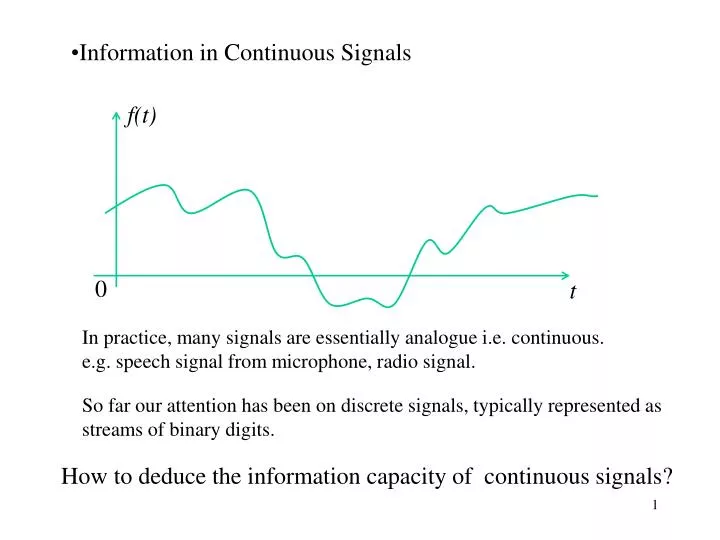
Information in Continuous Signals. f(t). 0. t. In practice, many signals are essentially analogue i.e. continuous. e.g. speech signal from microphone, radio signal. So far our attention has been on discrete signals, typically represented as streams of binary digits.

E N D
Information in Continuous Signals f(t) 0 t In practice, many signals are essentially analogue i.e. continuous. e.g. speech signal from microphone, radio signal. So far our attention has been on discrete signals, typically represented as streams of binary digits. How to deduce the information capacity of continuous signals?
Sampling Theorem Numbers of samples/s ≥2W (1/T ≥2W ), W Nyquist rate f(t) fs(t) T t f t 2T 3T 4T F(f) F (fs) f f -W W Spectrum of continuous signal Spectrum of sampled signal
Information capacity in continuous signal Information per second: R=(number of independent samples/s) × (maximum information per sample) number of independent samples/s =2W maximum information per sample in discrete signal? H=-Σp log p What is maximum information per sample in continuous signal? number of distinguishable levels =S/N For continuous signal, maximum information per second is usually denoted as Information Capacity C=2Wlog(S/N)=W log (SNR)
Relative Entropy of Continuous Signal Discrete systems Continuous systems Gaussian
Information Capacity of Continuous Signals Input (x) Output (y) Channel Power (S) Power (S+N) Information Capacity C=[H(y)-H(n)]×2W This leads to Ideal Communication Theorem C=Wlog(1+S/N) Theoretically information could be transmitted at a rate up to C with no net errors.
Transmission Media The physical medium of electronic transmission limits its achievable bit rate. It acts as a “filter” on the signal being transmitted.
Shannon’s Theorem Our phone line can carry frequencies between 300 Hz and 3300Hz unattenuated. The channel capacity C is C=W log2 (1+S/N) W is the bandwidth 3300-300=3000 Hz. S/N is the signal to noise ratio, typically 1000, which corresponds to 10 log10 (S/N) dB = 30dB. In our case C=30 kbs, corresponds well with a 28.8kbs modem.
Implications of the Ideal Theorem I=WTlog(1+SNR) bits in time T. A given amount of information can be transmitted by many combinations of W, T, SNR W 3 C=3 units T=1s 2 c a 1 b 60 10 SNR a. W=1, SNR=7, b. Half W S/N =63. Requires very large increase in power. c. Half S/N W1.5. Useful can halve power with only 50% increase in bandwidth.
Maximum Capacity for given transmitted Power C=W log (1+S/N) S/N0 nats =1.44S/N0 bits (about 3×10 ‾ ²¹ W required to transmit 1 bit.) C=Wlog(1+S/(N0 W)) , where N0 is noise power spectral density. Max value of C occurs for W ∞, and P/N 0 This suggests that power should be spread over a wide bandwidth and transmitted at as low P/N as possible for efficiency in power requirements.