1 / 126

File→ open→ select the samples.xls → open

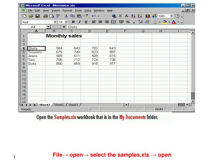
File→ open→ select the samples.xls → open. Click new tool from the standard tool bar. File → save as → select Microsoft excel 5.0/95 work book from save as type → click save. Help → Microsoft excel help → type advanced filters → click search.

belva
Télécharger la présentation

File→ open→ select the samples.xls → open

An Image/Link below is provided (as is) to download presentation Download Policy: Content on the Website is provided to you AS IS for your information and personal use and may not be sold / licensed / shared on other websites without getting consent from its author. Content is provided to you AS IS for your information and personal use only. Download presentation by click this link. While downloading, if for some reason you are not able to download a presentation, the publisher may have deleted the file from their server. During download, if you can't get a presentation, the file might be deleted by the publisher.

E N D

Presentation Transcript


  1. File→ open→ select the samples.xls → open

  2. Click new tool from the standard tool bar

  3. File → save as → select Microsoft excel 5.0/95 work book from save as type → click save

  4. Help → Microsoft excel help → type advanced filters → click search

  5. Tool → options → select General tab → in user name type Carla Banks

  6. Select B5 cell → type 521→ click any other cell

  7. Click on the gray area of the row 4

  8. Click on the undo tool from the standard tool bar

  9. Double click on the gray area between Row 2 and Row 3

  10. Select cell B2 → type Cost→ press Enter

  11. Click copy from the standard tool bar → select the Marketing worksheet → click paste from the standard tool bar

  12. Select the cell B3 → press the delete key from the keyboard

  13. Edit → select replace → type Jane Harris in the find what → type Tom Snow in replace with → click replace all

  14. Click the sort descending tool from the standard tool bar

  15. Right click on the sales worksheet → select insert → ok

  16. Right click on the Annuals worksheet → select move or copy → select Contracts from to book → select move to end from before sheet → ok

  17. = B5-B11

  18. A#NAME? Error message

  19. =B3*$C$1

  20. =sum(B2:B4)+$B$8

  21. Type = min (F5:F7) → press Enter

  22. =sum(B3:B9)

  23. =IF (B3>300, 10%, 0%)

  24. Click on increase decimal tool from the formatting tool bar

  25. Format → select cells → select currency from the category → select £ English (United Kingdom) → ok

  26. Click on the bold tool from the formatting tool bar

  27. Click the format painter tool from the standard tool bar → click on cell D3

  28. Format → select cells → select Alignment tab → in the orientation area move the red point up to the first point

  29. Select the range → insert → select chart → select pie in the chart type → click finish

  30. Click copy from standard tool bar → select the Conference workbook → click paste from the standard tool bar

  31. Click on the arrow in the chart type tool in the chart tool bar → select bar chart

  32. File → select page setup → select margins tab → type 2 in top box → ok

  33. File → select page setup→ delete number 4 and type 3→ ok

  34. View → select Header and Footer → click custom Header → click in the center section→ click on → ok → ok

  35. File → select page setup → select sheet tab → check the gridlines in the print section

  36. File → select print → ok

  37. File→ save as →change the name Expense Claim into Accounts→ok

  38. Click on the gray area of the column c

  39. Right click on the gray area → select delete

  40. Select cell B3→ press delete from the keyboard

  41. Right click on the sheet2 tab → select rename → type Costs

  42. Type = B4*C4 → press Enter

  43. A Circular Reference error message

  44. =sum(B3:B5)

  45. =sum(B2:D2)+$B$6

  46. The first X put it on 110 The second X put it on Apr The second X put it on pares

  47. File → print → in print what section → select Selection

  48. Type =sum (f5:f7) →press enter from the keyboard

  49. =count (B4:D10)

  50. =if (D7>10000, 7%, 0%)

More Related