Download
1 / 37
370 likes | 553 Vues
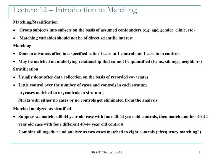
Lecture 12 – Introduction to Matching. Conditional logistic regression. Conditional logistic regression. Conditional logistic regression. Conditional logistic regression. Example. Example. Usual odds ratio and Mantel-Haenszel odds ratio adjusting for year of birth

E N D
Lecture 12 – Introduction to Matching BIOST 536 Lecture 12
Conditional logistic regression BIOST 536 Lecture 12
Conditional logistic regression BIOST 536 Lecture 12
Conditional logistic regression BIOST 536 Lecture 12
Conditional logistic regression BIOST 536 Lecture 12
Example BIOST 536 Lecture 12
Example • Usual odds ratio and Mantel-Haenszel odds ratio adjusting for year of birth • Standard logistic regression BIOST 536 Lecture 12
Example • Unconditional logistic regression adjusting for YOB BIOST 536 Lecture 12
Example BIOST 536 Lecture 12
Example • Conditional logistic regression stratified on YOBwith m cases : n controls for each YOB (“true stratification”) • In all the analyses, the OR and 95% CI are about the same due to the close frequency matching BIOST 536 Lecture 12
Conditional logistic regression BIOST 536 Lecture 12
1-1 matching BIOST 536 Lecture 12
1-1 matching BIOST 536 Lecture 12
1-1 matching BIOST 536 Lecture 12
1-1 matching BIOST 536 Lecture 12
Example BIOST 536 Lecture 12
Example • Not really what we want since we want to retain the matching and compare Gall (case) vs Gall (control) BIOST 536 Lecture 12
Example • Use small trick to get case and control value on the same line for Gall bladder disease BIOST 536 Lecture 12
Example • Can use matched case-control command (mcc) • Can get the OR easily and get confidence intervals and exact p-values based on the exact binomial distribution with null hypothesis p=0.50 and n = number discordant on exposure status • Easier to just use conditional logistic regression BIOST 536 Lecture 12
Example BIOST 536 Lecture 12
Example BIOST 536 Lecture 12
Example BIOST 536 Lecture 12
Example BIOST 536 Lecture 12
Example BIOST 536 Lecture 12
1-m matching BIOST 536 Lecture 12
1-m matching BIOST 536 Lecture 12
1-m matching BIOST 536 Lecture 12
Example BIOST 536 Lecture 12
Example BIOST 536 Lecture 12
Example BIOST 536 Lecture 12
Example BIOST 536 Lecture 12
Example BIOST 536 Lecture 12
Example BIOST 536 Lecture 12
Example BIOST 536 Lecture 12
Example BIOST 536 Lecture 12
Summary • 1-1 matching case-control • Only sets where the covariate is different between case and control supply information about that covariate • Cannot get absolute probabilities, just conditional probabilities • Missing value for the case or control will cause loss of the set • 1-m matching case-control • Only sets where the covariate is different between the case and at least one control will supply information about that covariate • Cannot get absolute probabilities, just conditional probabilities • Missing value for the case will cause loss of the set • Can use Wald and LR tests as before for model fitting BIOST 536 Lecture 12