Chap2 Image enhancement (Spatial domain)

1. Chap2 Image enhancement (Spatial domain)

2. Preprocessing • Why we need image enhancement? • Un-necessary noises • Defects caused by image acquisition • Uneven illumination: non-uniform • Lens: blurring object or background • Motion : blurring • Distortion: geometric distortion caused by lens • registration

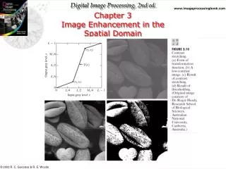
3. Chapter 2 Image Enhancement in the Spatial Domain 2.1 Background • Specific application—problem oriented • Trial and error is necessary • Spatial domain will be denoted by the expression g(x,y)=T[f(x,y)] • The simplest form of T: s=T(r) • Contrast stretching: (Fig. 3.2 (a)) • Thresholding function: binary image (Fig. 3.2) • Masks (filters, kernels, templates, windows) • Enhancement : mask processing or filtering 2.2 Some gray level transformations • Three basic types of functions used for image enhancement • Linear • logarithmic • Power-law

4. 2.2.1 Image negatives • Is obtained by using the negative transformation s=L-1-r • Produces the equivalent of a photographic negative • Suited for enhancing white or gray detail embedded in dark regions of an image 2.2.2 Log transformations • The general form of the log transformation : s=clog(1+r) • Expand the values of dark pixels while compressing the high-level values • Compress the dynamic range of images with large variations 2.2.3 Power-law transformation • The basic form: • Gamma correction • CRT device have an intensity-to-voltage response that is a power function • Produce images that are darker than intended • Is important if displaying an image accurately on a computer screen

5. Chapter 3 Image Enhancement in the Spatial Domain

6. Chapter 3 Image Enhancement in the Spatial Domain

7. Chapter 2 Image Enhancement in the Spatial Domain

8. Chapter 2 Image Enhancement in the Spatial Domain

9. Chapter 2 Image Enhancement in the Spatial Domain

10. Chapter 2 Image Enhancement in the Spatial Domain

11. Low r: wash-out in the background (Fig. 3.8 r=0.3) • High r: enhance a wash-out appearance (Fig. 3.9 r=0.5 areas are too dark) 2.2.4 Piecewise-linear transformation functions • Advantage: the form of piecewise functions can be arbitrary complex over the previous functions • Disadvantage: require considerably more user input • Contrast stretching • One of the simplest piecewise function • Increase the dynamic range of the gray levels in the image • A typical transformation: control the shape of the transformation • r1=r2 s1=0 and s2=L-1 • Gray level slicing • Highlight a specific range of gray levels • Display a high value for all gray levels in the range of interest and a low value for all other gray levels : produce a binary image

12. Continue • Brighten the desired range of gray levels, but preserves the background and gray level tonalities (Fig. 3.11) • The higher order bits (especially the top four) contain the majority of the visually significant data

13. Chapter 2 Image Enhancement in the Spatial Domain

14. Chapter 2 Image Enhancement in the Spatial Domain

15. Chapter 2 Image Enhancement in the Spatial Domain

16. Chapter 2 Image Enhancement in the Spatial Domain

17. 2.3 Histogram processing Histogram of a digital image with the gray levels in the range[0, L-1] • Low contrast: a narrow histogram, a dull, wash-out gray look • High contrast : cover a broader range of the gray scale and the distribution of pixels is not too far uniform, with very few vertical lines being much higher than the others • A great deal of details and high dynamic range 2.3.1 Histogram equalization • Histogram of S=T (r) 0 r1 • produce a level s for every pixel value in the original image, the transformation satisfies the following conditions: (1) T(r) is single-valued and monotonically increasing in the interval 0 r 1; and (2) 0 T ( r )  1 for 0 r 1 • r=T-1(s) 0 s 1

18. Chapter 2 Image Enhancement in the Spatial Domain

19. Chapter 2 Image Enhancement in the Spatial Domain

20. 3.4 Enhancement using arithmetic/logic operations • Image subtraction —g(x,y)=f(x,y)-h(x,y) • Masking • is referred to as ROI (region of interest) processing • Isolate an area for processing • Arithmetic operations • Addition: • Subtraction: • Multiplication: used to implement gray-level rather than binary • Division: • Logic operations • And: used for masking (Fig. 3.27) • Or:used for masking • Not operation: negative transformation • Also are used in conjunction with morphological operations

21. Chapter 3 Image Enhancement in the Spatial Domain

22. 2.4.1 Image subtraction • The difference between two images f(x,y) and h(x,y) is expressed as g(x,y)=f(x,y)-h(x,y) • Enhance the difference part of two images • Contrast stretching transformation—useful for evaluating the effect of setting to zero the lower-order planes (Fig. 3.28(d)) • Mask mode radiography (Fig 3.29) • Sort of scaling : solve image values outside form the range 0 to 255 (-255 to 255) • (1) Add 255 to every pixel and divide by 2: fast and simple to implement, but the full rang of the display may not be used • (2) more accuracy and full coverage of the 8-it range • The values of the minimum difference is obtained and its negative added to all the pixels in the difference image • All the pixels in the image are scaled to [0,255] by multiplying 255/Max 2.4.2 Image averaging • g(x,y)=f(x,y)+(x,y) (assume every pair of coordinates (x,y) the noise is uncorrelated and has zero average value)

23. Chapter 3 Image Enhancement in the Spatial Domain

24. Chapter 3 Image Enhancement in the Spatial Domain

25. Reduce the noise content by adding a set of noise images {gi(x,y)} • An image is formed by averaging K different noisy images • As k increases, the variability of the pixel values at each location (x,y) decreases • The image gi(x,y) must be registered in order to avoid the introduction of blurring • Use integrating capabilities of CCD or similar sensors for noise reduction by observing the same scene over long periods of time 3.5 Basics of spatial filtering • Sub-image: (filter, mask, kernel, template or window) • Frequency domain: • Spatial domain • Linear spatial filtering: is give by a sum of products of the filter coefficients R= • In general, linear filtering of an image with a filter mask of size MxN is given by g(x,y) • Convolving a mask with an image by pixel-by-pixel basis

26. Chapter 3 Image Enhancement in the Spatial Domain

27. Chapter 3 Image Enhancement in the Spatial Domain

28. Chapter 3 Image Enhancement in the Spatial Domain

29. Chapter 3 Image Enhancement in the Spatial Domain

30. 2.6 Smoothing spatialfilters • Used for blurring and for noise reduction • Blurring is used for removal of detail and bridging of small gaps in lines or curves 2.6.1 Smoothing linear filters • Averaging filter (low pass filter) • Replace the value of every pixel by the average of the gray levels in the neighborhood by the filter mask • Reduce sharp transition (such as random noise) • Blur edges • The average of the gray levels in the 3x3 neighborhoods • Averaging with limited data validity • only to pixels in the original image in a pre-defined interval of invalid data • Only if the computed brightness change of a pixel is in some pre-defined interval

31. Averaging according to inverse gradient • =Averaging using a rotation mask 2.6.2 Order Statistics filters (rank filters) • Nonlinear spatial filter based on ordering (ranking) • Median filter • Remove impulse noises (salt and pepper noises) • Represent 50 percent of a ranked set • Large clusters are affected considerably less • Min filter • Max filter--useful in finding the brightest points • Non-linear mean filter • Arithmetic mean • Harmonic mean • Geometric mean

32. Chapter 3 Image Enhancement in the Spatial Domain

33. Chapter 3 Image Enhancement in the Spatial Domain

34. Chapter 3 Image Enhancement in the Spatial Domain

35. 3.7 Sharpening spatial filter • Highlight fine detail or enhance detail • Enhance detail that has been blurred • Application ranging from electronic printing and medical imaging to industrial inspection • Can be accomplished by digital differentiation 3.7.1 Foundation • Sharpening filter based on first- and second-order derivatives • Definition for first derivatives • Must be zero in flat segment • Muse be nonzero at the onset of a gray level step or ramp • Must be nonzero along ramps • Def. of first derivate: • Produce “thick” edges • Has a strong response to gray-level step

36. Definition for second derivatives: is better suited than the first-derivative for image enhancement • Must be zero in flat areas • Muse be nonzero at the onset and end of a gray level step or ramp • Must be zero along ramps of constant slope • Def. Of a second order derivate: • Produces finer edges • Enhance fine detail much more than a first order derivate for example: a thin line • The stronger response at an isolated point • Has a transition form positive back to negative • Produces a double response to a gray-level step • Highlight the fundamental similarities and differences between first- and second- order derivatives (Fig. 3.38)

37. Chapter 3 Image Enhancement in the Spatial Domain

38. Chapter 3 Image Enhancement in the Spatial Domain

39. Chapter 3 Image Enhancement in the Spatial Domain

40. Chapter 3 Image Enhancement in the Spatial Domain

41. Chapter 3 Image Enhancement in the Spatial Domain

42. Approximate the magnitude of the gradient by using absolute values • Lost isotropic feature property • Vertical and horizontal edges preserve the isotropic properties only for multiples of 90 • Mask of odd sizes • Robert operator • Robert Ross-gradient operators • An approximation using absolute values (3.7-18) • Sobel operator • Use a weight value of 2 to achieve some smoothing by giving more importance to the center point • Constant or slowly varying shades are eliminated • Prewitt operator