Download
1 / 22
280 likes | 997 Vues
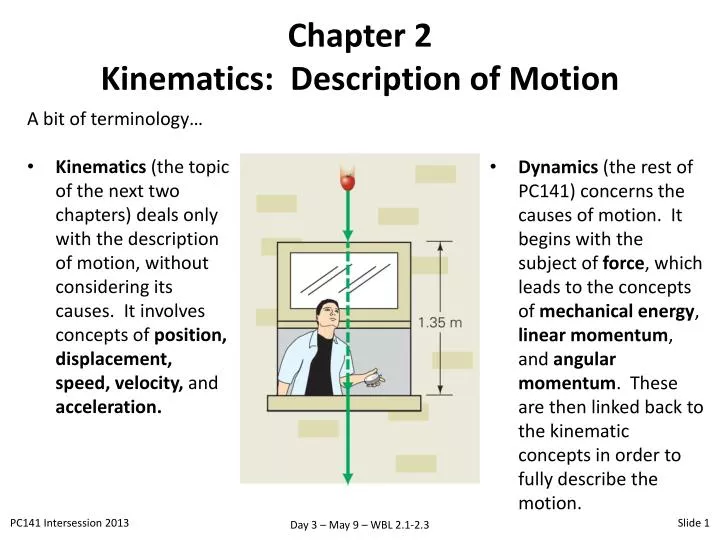
Chapter 2 Kinematics: Description of Motion. A bit of terminology … Kinematics (the topic of the next two chapters) deals only with the description of motion, without considering its causes. It involves concepts of position, displacement, speed, velocity, and acceleration .

E N D
Chapter 2Kinematics: Description of Motion • A bit of terminology… • Kinematics (the topic of the next two chapters) deals only with the description of motion, without considering its causes. It involves concepts of position, displacement, speed, velocity, and acceleration. • Dynamics(the rest of PC141) concerns the causes of motion. It begins with the subject of force, which leads to the concepts of mechanicalenergy, linearmomentum, and angular momentum. These are then linked back to the kinematic concepts in order to fully describe the motion.
2.1 Distance and Speed All motion involves changing an object’s position. In studying kinematics, we wish to analyze (or predict) where an object is (or will be) at various times. The simplest description of motion is the distance that an object travels, which is the total path length traversed in moving between two points. Distance depends not only on the position of the two points, but on the particular path taken during the trip. Distance is a scalar quantity(it has a magnitude – and units – but no direction). The text uses the symbol d to represent distance.
2.1 Distance and Speed When an object is in motion, it moves a certain position in a given amount of time. The relationship between these two parameters tells us the object’s speed. Average speed is the distance traveled divided by the time elapsed during the trip. Note that the bar over s is used to denote an average quantity, not to indicate a vector. We denote the start and end times of the trip as t1and t2, respectively. The time elapsed is notated as Δt =t2 – t1 (“Δ” is the Greek capital letter “delta”, which is used in the sciences to represent a “difference” or “change”). Then, As the ratio of a distance and a time, speed has SI units of m/s. Other common units are km/h and miles/h (often written mph).
2.1 Distance and Speed We can also define an instantaneous speeds as the speed at a particular moment in time. That is, it is the average speed in the limit as Δt approaches zero. The speedometer in a car shows instantaneous speed (more or less…all sensors have a finite “sensing time”, but it’s very short). Instantaneous speed is very important in calculus-based physics courses, but we won’t use it very often in PC141.
2.2 1D Displacement and Velocity For the remainder of this chapter, we will only consider motion in one dimension – that is, objects are constrained to move back and forth along a straight line. This may seem like a very restrictive view of the world, but it will turn out to be quite useful. ORIGIN To begin, we will label the straight line as the x-axis. The position of an object is a function of time, labeled x(t). Its value depends on where we place the origin, where x = 0. This location is entirely up to us.
2.2 1D Displacement and Velocity Displacement is the straight-line distance between two points, along with an indication of the direction (which is positive if x increases from the first point to the second, and negative if x decreases). The man in the figure has a displacement of +8 m if he walks from x1 to x2, where x1 = x(t1) and x2= x(t2). Mathematically, we write Since it has both a magnitude and a direction, displacement is a vector quantity.
2.2 1D Displacement and Velocity Velocity tells us both how fast an object is moving and in what direction. The average velocity between time t1 (when the object is at position x1) and time t2(when the object is at position x2) is Average velocity and average speed are not the same thing. For example, if you take a walk to the corner store and back, you might travel a total of 300 m in 5 minutes. Your speed is (300 m) / (300 s) = 1 m/s. However, since your starting position and ending position are the same, your displacement is Δx = 0, so your average velocity is zero.
2.2 Displacement and Velocity As with speed, we can also define an instantaneous velocityv as the velocity at a particular moment in time. That is, it is the average velocity in the limit as Δt approaches zero: Uniform motion is motion in which the velocity is constant (in both magnitude and direction). In uniform motion, the average velocity and instantaneous velocity are identical.
2.2 Displacement and Velocity Graphical analysis is often used in PC141 (and in most science courses). For 1D motion, we can plot position as a function of time,x vs. t. Then, the description of average velocity from slide 7 indicates that it is equal to the slope of this graph, . Thus, we see that a positive average velocity produces a graph with positive slope (slide 8), and a negative average velocity produces a graph with negative slope (below). If the velocity is constant, then the slope can never change. In this case, the graph is a straight line.
2.2 Displacement and Velocity If the velocity is not constant, then the graph is a curve. The plot below shows position vs. time for an object that speeds up, slows down, reverses direction, etc. We will discuss it in class.
2.3 Acceleration When an object’s velocity is not constant, we say that the object has a non-zero acceleration. The relationship between acceleration and velocity is identical to that between velocity and position. That is, acceleration is the time rate of change of velocity. The average acceleration is defined as SI units for acceleration are m/s2. Don’t waste too much time contemplating the concept of a “squared second”… the units merely refer to the fact that the ratio of a velocity to a time is measured as (m/s) / s. We can also express the instantaneous acceleration as
2.3 Acceleration Since velocity is a vector, so is acceleration. A change in velocity might indicate a change in speed, or a change in direction, or both. Either of these will produce a non-zero acceleration. The case of a change in speed (not direction) is shown below. The directions of velocity and acceleration and their relation to whether an object is “speeding up” or “slowing down” are rather confusing at first.
2.3 Acceleration In the figure, the positive direction (the direction of increasing x) is to the right. Since Δt is positive (it’s the difference between a later time and an earlier time), the sign of is identical to the sign of . We will discuss this figure in class.
2.3 Acceleration The case of a change in direction (not speed) is shown below on the left. We won’t analyze this one quite yet – since this motion takes place in 2 dimensions, we will save it for the next chapter. It is also possible to change both speed and direction, as shown on the right.
2.3 Acceleration In general, acceleration can be a function of time, a(t). However, when acceleration is constant, we can derive many simple relationships among acceleration, velocity, and position. The text implies that this case is examined “for simplicity”… I disagree! There are many examples of physical situations for which acceleration really is constant. In fact, much of PC141 is concerned with these situations. To begin, we need to adjust our notation a bit. Until now, we assumed that there were two specific times, t1 and t2, at which an object had position x1and x2 and velocity v1and v2. Here, we will change the initial conditions to t0 = 0, x0, and v0, and consider the final conditions as variables t, x, and v. Note that we can set the initial time to zero since only changes in time have any physical meaning.
2.3 Acceleration Next, we note that if acceleration is constant, then the average acceleration over a duration of time and the instantaneous acceleration at any particular time must be equal: . Rearranging our original equation for average acceleration, we have Then, rearranging once more, we find that In other words, when acceleration is constant, the velocity at any future time t is equal to the velocity at the initial time plus the product of acceleration and time.
2.3 Acceleration We see from the previous equation that the function is a straight line, with slope and intercept .
Problem #1: Graphical Analysis WBL LP 2.6
Problem #2: Deceleration WBL LP 2.11
Problem #4: Nerve Conduction The human body contains different types of nerves, and the speed at which impulses travel along these nerves strongly depends on the particular type. The sensation of touch relies on Aα receptors, which conduct impulses at roughly 100 m/s. The sensation of pain relies on C receptors, which conduct impulses at about 0.6 m/s. Assume that your left big toe is 160 cm from your brain. What is the time lag between realizing that you’ve stubbed your toe and feeling the resulting pain? Solution: In class
Problem #5: Train Trip WBL EX 2.7 A train makes a round trip on a straight, level track. The first half of the trip is 300 km, and is traveled at a speed of 75 km/h. After a 0.50-hour layover, the train returns to its original location at a speed of 85 km/h. What is the train’s (a) average speed, and (b) average velocity? Solution: In class