Download
1 / 35
370 likes | 715 Vues
Quick Response in Manufacturer-Retailer Channels. Ananth V. Iyer • Mark E. Bergen. Presented By Evren Körpeoğlu. Quick Response. Quick Response is a strategy focusing on providing shorter lead times. It enables orders to be placed closer to the start of the selling season.

E N D
Quick Response in Manufacturer-Retailer Channels Ananth V. Iyer • Mark E. Bergen Presented By Evren Körpeoğlu
Quick Response • Quick Response is a strategy focusing on providing shorter lead times. • It enables orders to be placed closer to the start of the selling season.
Quick Response & Apparel Industry • Used mainly in Apparel Industry, because of; • Long lead times between order placement and delivery of product.
Quick Response • To Reduce the lead times; • Information Sharing using EDI • Logistics improvements • Increased use of Air Freight • Point of sale scanners and barcoding • Improved manufacturing methods such as laser fabric cutting or modular sewing cells
Is it Pareto Improving? • Do both the manufacturer and the retailer benefit from QR? • This paper investigates the effect of QR and how to make it become Pareto improving.
Model Structure • Old System: • L = Lead Time (5 to 8 months) • QR System: • L2 = Lead Time (2 to 5 months) • L2≤L • L2= L – L1
Demand Structure • We have two levels of demand uncertainity: • Uncertainity of the number of people who come to the store and their propensity to buy • Uncertainity about mean demand
Demand Structure before QR • N(θ,σ2): distribution of demand during season assuming that we know meand demand N(μ,τ2): mean demand estimation • m(x)~N(μ,τ2+σ2) → demand distribution at time 0
Demand Structure after QR • Data collected during period L1 is used to estimate the demand of the season. • If the demand in period L1 is d1, then: m(x|d1)~N(μ(d1), σ2 + 1/Ρ)
QR and the Channel Model Parameters: c: Cost per unit to buy product from manufacturer ∏: Goodwill cost per unit h: holding cost per unit of product left over at the the end of the season w: production cost per unit r: retailer’s revenue per unit
The Old System Expected Revenues Holding Costs Goodwill Costs
The Old System Optimum initial inventory: Optimal service level (s):
The Old System Maximum Expected Profit:
The Old System Expected Quantity Sold: Expected Quantity Left over:
QR System • Retailer’s inventory choice involves two steps: • Observe the demand during L1 and use it to estimate seasonal demand • Choose optimal inventory to maximize expected profits with estimated demand. The demand before season,d1, directly affects this choice.
QR System Optimum initial inventory: Maximum Expected Profit:
QR System Expected Quantity Sold: Expected Quantity Left over:
Old System vs QR System Since: • EIQR-sold ≥ EIold-sold • EIQR-left ≤ EIold-left
Old System vs QR System Expected Manufacturer Profit in old system: Expected Manufacturer Profit in QR system:
When is QR Pareto Improving? Lemma 1: • If s≤0.5 then under QR we have an increase in manufacturer and retailer expected profits because Z(s) < 0 • Thus, under low service levels, QR is pareto improving.
When is QR Pareto Improving? In the case that manufacturer pays a salvage credit per unit, if this credit is large enough, then QR will be pareto improving even if s≥0.5
When is QR Pareto Improving? Lemma 2: • If s≥0.5 then under QR we have an increase in expected retailer profits but a decrease in expected manufacturer profits
Other Methods... • Commitments using service level • Commitments regarding the wholesale price • Volume commitments across products
Commitments using service level • After QR, retailer may use a higher service level but it is not beneficial for the manufacturer • Since the increase in service level can not be shown in the model, the goodwill costs are changed.
Commitments using service level Theorem 1. If s≥0.5, d=σ/τ and then increasing ∏ to ∏’=(s’(r+h)+c-r)/(1-s’) and s’ such that Z(s’)=Z(s)/y makes QR Pareto improving.
Commitments using service level Lemma 3. If s≥0.5, d=σ/τ and then increasing ∏ to ∏’=(s’(r+h)+c-r)/(1-s’) and s’ such that Z(s’)=Z(s)/y, results in EIQR-sold(s’) ≥ Iold-sold and EIQR-left (s’)≤ Iold-left
Commitments using service level Other ways in using service level; • Contractual commitment between manufacturer and retailer to provide high service level • Use of cooperative advertising that uses service level guarantee • Increasing the goodwill cost
Wholesale Price Quantity Discounts: • If manufacturer forces retailer pay c1>c if the quantity purchased is smaller than the Iold, and c if it is larger than Iold, manufacturer may benefit from QR. Lemma 4: There exists a quantity discount scheme that makes QR Pareto improving
Wholesale Price Lemma 5: There exists a wholesale price c* that depends on system parameters such that if c≥c*, then there exists no flat wholeslae price commitments that can make QR Pareto improving.
Volume Commitments across Products • Assuming we have M products, the buyer should have a commitment that the total amount of purchased products will be as much as before the QR.
Volume Commitments across Products Lemma 6: The impact of a volume commitment of I(M), which is initial inventory across M products, on expected profit for the retailer is given by Thus a volume commitment of M(μ+Zs√σ2+ τ2) across M products makes QR Pareto improving.
Volume Commitments across Products Volume commitment maintains manufacturer’s profit but genrate an expected service level which is below that is required for service level commitments
Volume Commitments across Products Lemma 7: The expected service level s(M) under a volume commitment of MIold across M products, s(M), is s≤S(M)≤s’, where is s’ is defined as in Theorem 1
Conclusion • Impact of a channel view on Quick Response for fashion apparel industry is examined. • Classical inventory model are used to show these effects. • Three ways for Pareto improving are consider: service level, price and volume commitments.
THANK YOU FOR LISTENING!... Comments & Questions