parallel computing: overview
330 likes | 715 Vues
Introduction to Parallel Computing. Why we need parallel computingHow such machines are builtHow we actually use these machines. New Applications. Clock Speeds. . Clock Speeds. When the PSC went from a 2.7 GFlop Y-MP to a 16 GFlop C90, the clock only got 50% faster. The rest of the speed increase was due to increased use of parallel techniques:More processors (8 ? 16)Longer vector pipes (64 ? 128)Parallel functional units (2).

parallel computing: overview
E N D
Presentation Transcript
1. Parallel Computing: Overview John Urbanic
urbanic@psc.edu
3. New Applications
4. Clock Speeds
5. Clock Speeds When the PSC went from a 2.7 GFlop Y-MP to a 16 GFlop C90, the clock only got 50% faster. The rest of the speed increase was due to increased use of parallel techniques:
More processors (8 ? 16)
Longer vector pipes (64 ? 128)
Parallel functional units (2)
6. Clock Speeds So, we want as many processors working together as possible. How do we do this? There are two distinct elements:
Hardware
vendor does this
Software
you, at least today
7. Amdahl�s Law How many processors can we really use?
Let�s say we have a legacy code such that is it only feasible to convert half of the heavily used routines to parallel:
8. Amdahl�s Law If we run this on a parallel machine with five processors:
Our code now takes about 60s. We have sped it up by about 40%. Let�s say we use a thousand processors:
We have now sped our code by about a factor of two.
9. Amdahl�s Law This seems pretty depressing, and it does point out one limitation of converting old codes one subroutine at a time. However, most new codes, and almost all parallel algorithms, can be written almost entirely in parallel (usually, the �start up� or initial input I/O code is the exception), resulting in significant practical speed ups. This can be quantified by how well a code scales which is often measured as efficiency.
10. Shared Memory Easiest to program. There are no real data distribution or communication issues. Why doesn�t everyone use this scheme?
Limited numbers of processors (tens) � Only so many processors can share the same bus before conflicts dominate.
Limited memory size � Memory shares bus as well. Accessing one part of memory will interfere with access to other parts.
11. Distributed Memory Number of processors only limited by physical size (tens of meters).
Memory only limited by the number of processors time the maximum memory per processor (very large). However, physical packaging usually dictates no local disk per node and hence no virtual memory.
Since local and remote data have much different access times, data distribution is very important. We must minimize communication.
12. Common Distributed Memory Machines CM-2
CM-5
T3E
Workstation Cluster
SP3
TCS
13. Common Distributed Memory Machines While the CM-2 is SIMD (one instruction unit for multiple processors), all the new machines are MIMD (multiple instructions for multiple processors) and based on commodity processors.
SP-2 POWER2
CM-5 SPARC
T3E Alpha
Workstations Your Pick
TCS Alpha
Therefore, the single most defining characteristic of any of these machines is probably the network.
14. Latency and Bandwidth Even with the "perfect" network we have here, performance is determined by two more quantities that, together with the topologies we'll look at, pretty much define the network: latency and bandwidth. Latency can nicely be defined as the time required to send a message with 0 bytes of data. This number often reflects either the overhead of packing your data into packets, or the delays in making intervening hops across the network between two nodes that aren't next to each other.
Bandwidth is the rate at which very large packets of information can be sent. If there was no latency, this is the rate at which all data would be transferred. It often reflects the physical capability of the wires and electronics connecting nodes.
15. Token-Ring/Ethernet with Workstations
16. Complete Connectivity
17. Super Cluster / SP2
18. CM-2
19. Binary Tree
20. CM-5 Fat Tree
21. INTEL Paragon (2-D Mesh)
22. 3-D Torus T3E has Global Addressing hardware, and this helps to simulate shared memory.
Torus means that �ends� are connected. This means A is really connected to B and the cube has no real boundary.
23. TCS Fat Tree
24. Data Parallel Only one executable.
Do computation on arrays of data using array operators.
Do communications using array shift or rearrangement operators.
Good for problems with static load balancing that are array-oriented SIMD machines.
Variants:
FORTRAN 90
CM FORTRAN
HPF
C*
CRAFT Strengths:
Scales transparently to different size machines
Easy debugging, as there I sonly one copy of coed executing in highly synchronized fashion
Weaknesses:
Much wasted synchronization
Difficult to balance load
25. Data Parallel � Cont�d Data Movement in FORTRAN 90
26. Data Parallel � Cont�d Data Movement in FORTRAN 90
27. Data Parallel � Cont�d When to use Data Parallel
Very array-oriented programs
FEA
Fluid Dynamics
Neural Nets
Weather Modeling
Very synchronized operations
Image processing
Math analysis
28. Work Sharing Splits up tasks (as opposed to arrays in date parallel) such as loops amongst separate processors.
Do computation on loops that are automatically distributed.
Do communication as a side effect of data loop distribution. Not important on shared memory machines.
If you have used CRAYs before, this of this as �advanced multitasking.�
Good for shared memory implementations. Strengths:
Directive based, so it can be added to existing serial codes
Weaknesses:
Limited flexibility
Efficiency dependent upon structure of existing serial code
May be very poor with distributed memory.
Variants:
CRAFT
Multitasking
29. Work Sharing � Cont�d When to use Work Sharing
Very large / complex / old existing codes: Gaussian 90
Already multitasked codes: Charmm
Portability (Directive Based)
(Not Recommended)
30. Load Balancing An important consideration which can be controlled by communication is load balancing:
Consider the case where a dataset is distributed evenly over 4 sites. Each site will run a piece of code which uses the data as input and attempts to find a convergence. It is possible that the data contained at sites 0, 2, and 3 may converge much faster than the data at site 1. If this is the case, the three sites which finished first will remain idle while site 1 finishes. When attempting to balance the amount of work being done at each site, one must take into account the speed of the processing site, the communication "expense" of starting and coordinating separate pieces of work, and the amount of work required by various pieces of data.
There are two forms of load balancing: static and dynamic.
31. Load Balancing � Cont�d Static Load Balancing
In static load balancing, the programmer must make a decision and assign a fixed amount of work to each processing site a priori.
Static load balancing can be used in either the Master-Slave (Host-Node) programming model or the "Hostless" programming model.
32. Load Balancing � Cont�d Static Load Balancing yields good performance when:
homogeneous cluster
each processing site has an equal amount of work
Poor performance when:
heterogeneous cluster where some processors are much faster (unless this is taken into account in the program design)
work distribution is uneven
33. Load Balancing � Cont�d Dynamic Load Balancing
Dynamic load balancing can be further divided into the categories:
task-orientedwhen one processing site finishes its task, it is assigned another task (this is the most commonly used form).
data-orientedwhen one processing site finishes its task before other sites, the site with the most work gives the idle site some of its data to process (this is much more complicated because it requires an extensive amount of bookkeeping).
Dynamic load balancing can be used only in the Master-Slave programming model.
ideal for:
codes where tasks are large enough to keep each processing site busy
codes where work is uneven
heterogeneous clusters