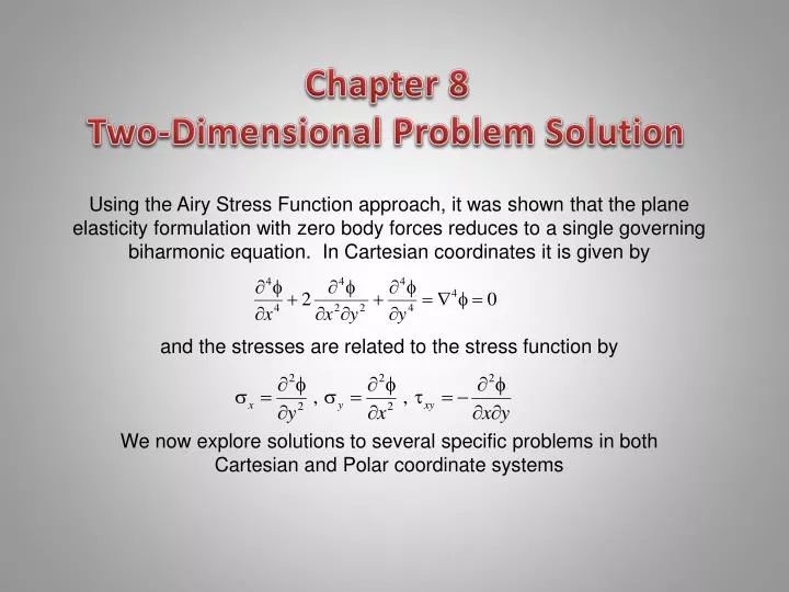
Chapter 8 Two-Dimensional Problem Solution

1. Chapter 8 Two-Dimensional Problem Solution Using the Airy Stress Function approach, it was shown that the plane elasticity formulation with zero body forces reduces to a single governing biharmonic equation. In Cartesian coordinates it is given by and the stresses are related to the stress function by We now explore solutions to several specific problems in both Cartesian and Polar coordinate systems

2. Cartesian Coordinate Solutions Using Polynomials In Cartesian coordinates we choose Airy stress function solution of polynomial form where Amn are constant coefficients to be determined. This method produces polynomial stress distributions, and thus would not satisfy general boundary conditions. However, we can modify such boundary conditions using Saint-Venant’s principle and replace a non-polynomial condition with a statically equivalent loading. This formulation is most useful for problems with rectangular domains, and is commonly based on the inverse solution concept where we assume a polynomial solution form and then try to find what problem it will solve. Noted that the three lowest order terms with m + n  1do not contribute to the stresses and will therefore be dropped. It should be noted that second order terms will produce a constant stress field, third-order terms will give a linear distribution of stress, and so on for higher-order polynomials. Terms with m + n  3will automatically satisfy the biharmonic equation for any choice of constants Amn. However, for higher order terms, constants Amn will have to be related in order to have the polynomial satisfy the biharmonic equation.

3. Example 8.1 Uniaxial Tension of a Beam Displacement Field (Plane Stress) Stress Field Boundary Conditions: Since the boundary conditions specify constant stresses on all boundaries, try a second-order stress function of the form The first boundary condition implies that A02 = T/2, and all other boundary conditions are identically satisfied. Therefore the stress field solution is given by . . . Rigid-Body Motion “Fixity conditions”needed to determine RBM terms

4. Example 8.2 Pure Bending of a Beam Stress Field Displacement Field (Plane Stress) Boundary Conditions: Expecting a linear bending stress distribution, try second-order stress function of the form Moment boundary condition implies that A03= -M/4c3, and all other boundary conditions are identically satisfied. Thus the stress field is “Fixity conditions”to determine RBM terms:

5. Example 8.2 Pure Bending of a BeamSolution Comparison of Elasticity with Elementary Mechanics of Materials Elasticity Solution Mechanics of Materials Solution Uses Euler-Bernoulli beam theory to find bending stress and deflection of beam centerline Two solutions are identical, with the exception of the x-displacements

6. Example 8.3 Bending of a Beam by Uniform Transverse Loading Stress Field Boundary Conditions: BC’s

7. Example 8.3 Beam ProblemStress Solution Comparison of Elasticity with Elementary Mechanics of Materials Elasticity Solution Mechanics of Materials Solution Shear stresses are identical, while normal stresses are not

8. Example 8.3 Beam ProblemNormal Stress Comparisons of Elasticity with Elementary Mechanics of Materials x – Stress at x=0 y - Stress Maximum difference between the two theories is wand this occurs at the top of the beam. Again this difference will be negligibly small for most beam problems where l >> c. These results are generally true for beam problems with other transverse loadings. Maximum differences between the two theories exist at top and bottom of beam, and actual difference in stress values is w/5. For most beam problems where l>> c, the bending stresses will be much greater than w, and thus the differences between elasticity and strength of materials will be relatively small.

9. Example 8.3 Beam ProblemNormal Stress Distribution on Beam Ends End stress distribution does not vanish and is nonlinear but gives zero resultant force.

10. Example 8.3 Beam Problem Displacement Field (Plane Stress) Choosing Fixity Conditions Strength of Materials: Good match for beams where l >> c

11. Cartesian Coordinate Solutions Using Fourier Methods A more general solution scheme for the biharmonic equation may be found using Fourier methods. Such techniques generally use separation of variables along with Fourier series or Fourier integrals. Choosing

12. Example 8.4 Beam with Sinusoidal Loading Stress Field Boundary Conditions:

13. Example 8.4 Beam Problem Bending Stress

14. Example 8.4 Beam Problem Displacement Field (Plane Stress) For the case l >> c Strength of Materials

15. Example 8.5 Rectangular Domain with Arbitrary Boundary Loading Must use series representation for Airy stress function to handle general boundary loading. Boundary Conditions Use Fourier series theory to handle general boundary conditions, and this generates a doubly infinite set of equations to solve for unknown constants in stress function form. See text for details

16. S R y  r  x Polar Coordinate FormulationAiry Stress Function Approach  = (r,θ) Airy Representation Biharmonic Governing Equation Traction Boundary Conditions

17. Polar Coordinate FormulationPlane Elasticity Problem Strain-Displacement Hooke’s Law

18. General Solutions in Polar CoordinatesMichell Solution Choosing the case where b = in, n = integer gives the general Michell solution We will use various terms from this general solution to solve several plane problems in polar coordinates

19. Axisymmetric Solutions Stress Function Approach:=(r) Navier Equation Approach:u=ur(r)er (Plane Stress or Plane Strain) Gives Stress Forms Displacements - Plane Stress Case Underlined terms represent rigid-body motion • a3term leads to multivalued behavior, and is not found following the displacement formulation approach • Could also have an axisymmetric elasticity problem using  =a4 which gives r =  = 0 andr= a4/r  0, see Exercise 8-14

20. Example 8.6 Thick-Walled Cylinder Under Uniform Boundary Pressure General Axisymmetric Stress Solution Boundary Conditions Using Strain Displacement Relations and Hooke’s Law for plane strain gives the radial displacement

21. r1/r2 = 0.5 Dimensionless Stress θ/p r /p r/r2 Dimensionless Distance, r/r2 Example 8.6 Cylinder Problem ResultsInternal Pressure Only Thin-Walled Tube Case: Matches with Strength of Materials Theory

22. Special Cases of Example 8-6 Stress Free Hole in an Infinite Medium Under Equal Biaxial Loading at Infinity Pressurized Hole in an Infinite Medium

23. Example 8.7 Infinite Medium with a Stress Free Hole Under Uniform Far Field Loading Boundary Conditions Try Stress Function

24. Example 8.7 Stress Results

25. Superposition of Example 8.7Biaxial Loading Cases T2 T1 T1 T2 Tension/Compression Case T1 = T , T2 = -T Equal Biaxial Tension Case T1 = T2 = T

26. Review Stress Concentration FactorsAround Stress Free Holes K = 2 K = 3 = K = 4

27. Stress Concentration Around Stress Free Elliptical Hole – Chapter 10 Maximum Stress Field

28. Stress Concentration Around Stress Free Hole in Orthotropic Material – Chapter 11

29. 2-D ThermoelasticStress Concentration Problem Uniform Heat Flow Around Stress Free Insulation Hole – Chapter 12 Stress Field Maximum compressive stress on hot side of hole Maximum tensile stress on cold side Steel Plate:E = 30Mpsi (200GPa) and = 6.5in/in/oF(11.7m/m/oC), qa/k= 100oF (37.7oC), the maximum stress becomes 19.5ksi (88.2MPa)

30. Nonhomogeneous Stress Concentration Around Stress Free Hole in a Plane Under Uniform Biaxial Loading with Radial Gradation of Young’s Modulus – Chapter 14

31. Two Dimensional Case:(r,/2)/S Three Dimensional Case:z(r,0)/S ,  = 0.3 Three Dimensional Stress Concentration Problem – Chapter 13 Normal Stress on the x,y-plane (z = 0)

32. Wedge Domain Problems Use general stress function solution to include terms that are bounded at origin and give uniform stresses on the boundaries Quarter Plane Example ( = 0 and  = /2)

33. Half-Space ExamplesUniform Normal Stress Over x 0 Boundary Conditions Try Airy Stress Function Use BC’s To Determine Stress Solution

34. Half-Space Under Concentrated Surface Force System (Flamant Problem) Boundary Conditions Try Airy Stress Function Use BC’s To Determine Stress Solution

35. Flamant Solution Stress ResultsNormal Force Case or in Cartesian components y = a

36. Flamant Solution Displacement ResultsNormal Force Case Note unpleasant feature of 2-D model that displacements become unbounded as r  On Free Surface y = 0

37. Comparison of Flamant Results with 3-D Theory - Boussinesq’s Problem Cartesian Solution Free Surface Displacements Cylindrical Solution Corresponding 2-D Results 3-D Solution eliminates the unbounded far-field behavior

38. Half-Space Under Uniform Normal Loading Over –axa dY= pdx = prd/sin

39. max - Contours Half-Space Under Uniform Normal Loading - Results

40. Generalized Superposition MethodHalf-Space Loading Problems

41. Photoelastic Contact Stress Fields

42. Notch/Crack Problem Try Stress Function: Boundary Conditions: At Crack Tip r 0: Finite Displacements and Singular Stresses at Crack Tip1<  <2  = 3/2

43. Notch/Crack Problem Results Transform to  Variable • Note special singular behavior of stress field O(1/r) • A and B coefficients are related to stress intensity factors and are useful in fracture mechanics theory • A terms give symmetric stress fields – Opening or Mode I behavior • B terms give antisymmetric stress fields – Shearing or Mode II behavior

44. Mode I (Maximum shear stress contours) Mode II (Maximum shear stress contours) ExperimentalPhotoelasticIsochromaticsCourtesy of URI Dynamic Photomechanics Laboratory Crack Problem ResultsContours of Maximum Shear Stress

45. Mode III Crack Problem – Exercise 8-32 Anti-Plane Strain Case z - Stress Contours Stresses Again

46. Curved Beam Under End Moments

47. Theory of Elasticity Strength of Materials Dimensionless Stress, a/P  = /2 b/a = 4 Dimensionless Distance, r/a Curved Cantilever Beam P  r a b

48. Disk Under Diametrical Compression P D = P Flamant Solution (1) + + Radial Tension Solution (3) Flamant Solution (2)

49. Disk Problem – Superposition of Stresses

50. Disk Problem – Results x-axis (y = 0) y-axis (x = 0)