Download
1 / 49
490 likes | 621 Vues
Statistical inference for epidemics on networks. PD O’Neill, T Kypraios ( Mathematical Sciences, University of Nottingham ). Sep 2011. ICMS, Edinburgh. Outline 1. Orientation 2. Inference for epidemics 3. Network models 4. Inference for network models 5. Open problems. Sep 2011.

E N D
Statistical inference for epidemics on networks PD O’Neill, T Kypraios (Mathematical Sciences, University of Nottingham) Sep 2011 ICMS, Edinburgh
Outline 1. Orientation 2. Inference for epidemics 3. Network models 4. Inference for network models 5. Open problems Sep 2011 ICMS, Edinburgh
Outline1. Orientation 2. Inference for epidemics 3. Network models 4. Inference for network models 5. Open problems Sep 2011 ICMS, Edinburgh
The basic problem Given data on a network and an infectious disease, can model parameters be inferred? 1. Orientation Sep 2011 ICMS, Edinburgh
The basic problem • Data • Can be partial or complete for network • Usually partial for disease • Can be multi-scale • May be longitudinal or not 1. Orientation Sep 2011 ICMS, Edinburgh
The basic problem • Model • Can be for the network • Can be for the disease • Can be both 1. Orientation Sep 2011 ICMS, Edinburgh
Outline 1. Orientation2. Inference for epidemics 3. Network models 4. Inference for network models 5. Open problems Sep 2011 ICMS, Edinburgh
2. Inference for epidemics • Consider Erdös-Renyi random graph on N vertices. • Let p = Prob(two edges connected) • Run an SIR model on graph: • Infection rate = β, Removal rate = γ Inference for network and disease given partial temporal data Sep 2011 ICMS, Edinburgh
2. Inference for epidemics Given complete observation of removal process, we wish to infer p, β and γ i.e. find posterior density (p, β, γ | data) Inference for network and disease given partial temporal data Sep 2011 ICMS, Edinburgh
2. Inference for epidemics Bayes’ Theorem gives (p, β, γ | data) (data | p, β, γ) (p, β, γ) However, the likelihood (data | p, β, γ) is intractable in practice. Inference for network and disease given partial temporal data Sep 2011 ICMS, Edinburgh
2. Inference for epidemics One solution is to augment the parameter space to include the unobserved infection events. This leads to a tractable likelihood, and the resulting posterior density can be explored using MCMC methods. Inference for network and disease given partial temporal data Sep 2011 ICMS, Edinburgh
2. Inference for epidemics • Britton & O’Neill (2002) – basic idea • Neal & Roberts (2005) – improved computational aspects • Ray & Marzouk (2008) – extended to two populations • Groendyke, Welch & Hunter (2011a) – SEIR model Inference for network and disease given partial temporal data Sep 2011 ICMS, Edinburgh
2. Inference for epidemics • Groendyke, Welch & Hunter (2011b) – More general network model where • pjk = function of covariates of j, k and (j,k) • but edges are still independent Inference for network and disease given partial temporal data Sep 2011 ICMS, Edinburgh
2. Inference for epidemics General comment – this estimation problem often leads to parameter identifiability issues. e.g. A highly connected network and low-infectivity disease, or a sparse network and high-infectivity disease? Inference for network and disease given partial temporal data Sep 2011 ICMS, Edinburgh
2. Inference for epidemics • Data tell us which individuals become infected and who is connected to whom. • Again the likelihood is intractable. • Augment data with network of infectious contacts (Demiris & O’Neill 2005; O’Neill 2009; van Boven et al. 2010). Inference for disease given final outcome data and network data Sep 2011 ICMS, Edinburgh
Outline 1. Orientation 2. Inference for epidemics3. Network models 4. Inference for network models 5. Open problems Sep 2011 ICMS, Edinburgh
3. Network models Most real-life networks require more general models which can incorporate a wide range of features. e.g. transitivity, homophily, self-organization, … Sep 2011 ICMS, Edinburgh
3. Network models • Basic idea: • Directed edges have covariates X(i,j) • Each vertex has a position in multivariate social space Z(i). • Edge prob(i,j) = f( X(i,j), | Z(i) – Z(j) | ) . • Z(i)’s are i.i.d. (e.g. Gaussian mixture). Latent position cluster models (Handcock, Raftery & Tantrum, 2007) Sep 2011 ICMS, Edinburgh
3. Network models Key point is that edge probabilities are conditionally (upon the Z(i)’s) independent. Given data on observed edges, inference can be carried out using MCMC or even ML. Latent position cluster models (Handcock, Raftery & Tantrum, 2007) Sep 2011 ICMS, Edinburgh
3. Network models Very widely used class of models in social network literature. Can incorporate many features of interest. Exponential Random Graph Models (Frank & Strauss, 1986) Sep 2011 ICMS, Edinburgh
3. Network models Let Y be a random N N adjacency matrix: Y(i,j) = 1 if edge from i to j is present, 0 if not. For Y=y, i = 1,…,m, s(i,y) denotes a summary statistic of y (e.g. number of edges, triangles, 3-stars, ….) Exponential Random Graph Models Sep 2011 ICMS, Edinburgh
3. Network models Then the ERGM is defined by ( y | ) = exp ( i (i) s(i,y) ) / z() Where = ((1), …, (m)) is a real m-vector, z() = y exp ( i (i) s(i,y) ) Exponential Random Graph Models Sep 2011 ICMS, Edinburgh
3. Network models Example: N=3, s(1,y) = # edges, s(2,y) = # triangles 8 possible graphs (4 up to isomorphism) Exponential Random Graph Models Sep 2011 ICMS, Edinburgh
3. Network models • ( y | ) 1 e(1) e2(1)e3(1)+ (2) • z() = 1 + 3e(1) + 3e2(1) + e3(1)+ (2) Exponential Random Graph Models Sep 2011 ICMS, Edinburgh
3. Network models (i) > 0 promotes s(i,y) (i) < 0 inhibits s(i,y) e.g. in the example (1) > 0 promotes edges (1) < 0 inhibits edges Exponential Random Graph Models Sep 2011 ICMS, Edinburgh
3. Network models Often see near-degeneracy in ERGMs in the sense that small number of graphs y are far more likely than all the others. Exponential Random Graph Models Sep 2011 ICMS, Edinburgh
3. Network models • =(2,1) • ( y | ) 0.001 0.017 0.128 0.854 Exponential Random Graph Models Sep 2011 ICMS, Edinburgh
3. Network models A key computational problem with ERGMs is that z() = y exp ( i (i) s(i,y) ) is intractable unless N is very small. Exponential Random Graph Models Sep 2011 ICMS, Edinburgh
Outline 1. Orientation 2. Inference for epidemics 3. Network models4. Inference for network models 5. Open problems Sep 2011 ICMS, Edinburgh
4. Inference for network models • Options include: • Maximum pseudolikelihood – not that good in general • Monte Carlo ML estimation – various practical problems Exponential Random Graph Models Sep 2011 ICMS, Edinburgh
4. Inference for network models Standard MCMC cannot be used since the posterior density is “doubly intractable”: (|y) (y|) () = f(y|) () / z() i.e. the likelihood itself is only known up to proportionality (know f(y|), not z() ). Exponential Random Graph Models Sep 2011 ICMS, Edinburgh
4. Inference for network models One option (Möller et al., 2006) is to augment the parameter space to include a new variable on the data space – call this x – and then work with the augmented posterior density ( x, | y). Exponential Random Graph Models Sep 2011 ICMS, Edinburgh
4. Inference for network models ( x, | y) = ( x | , y) ( | y) = ( x | , y) f(y | ) () / z() (y) Exponential Random Graph Models Sep 2011 ICMS, Edinburgh
4. Inference for network models A Metropolis-Hastings algorithm requires a proposal to update (x,). If we can draw a random graph from the distribution of y given then we may choose q(x*,* | x,) = q(x* | ) q (* |) = f (x * | ) q (* |) / z() Exponential Random Graph Models Sep 2011 ICMS, Edinburgh
4. Inference for network models The resulting M-H acceptance probability ratio is then of the form ( x* | *, y) f(y | *) f(x| ) q( |*) (*) ( x | , y) f(y | ) f(x*| ) q(* |) () and z() is not required. Exponential Random Graph Models Sep 2011 ICMS, Edinburgh
4. Inference for network models The crucial assumption is the ability to sample from the original ERGM given ; in practice this is usually achieved using MCMC. Variations of the Möller method have been developed – essentially choices of ( x | , y). Exponential Random Graph Models Sep 2011 ICMS, Edinburgh
Outline 1. Orientation 2. Inference for epidemics 3. Network models 4. Inference for network models5. Open problems Sep 2011 ICMS, Edinburgh
5. Open Problems 1. Simulating random graphs from ERGMs? • MCMC is considered as the gold-standard method to draw from (y|) for given -- essential in order to draw inference for . • Is it possible to use an exact algorithm instead? For instance, rejection sampling? What would be a good proposal distribution? Efficiency? Sep 2011 ICMS, Edinburgh
5. Open Problems 2. Approximate inference for ERGMs? • Bayesian inference for ERGMs often relies on advanced MCMC algorithms (Cairo and Friel, 2010) • Alternatively, one can resort to approximate methods which are easier to implement. Sep 2011 ICMS, Edinburgh
5. Open Problems 2. Approximate inference for ERGMs? • Data y; parameter ; target distribution (|y). • Consider the following algorithm: • Draw * from the prior (). • Simulate data y* from (y*|*) • If y* = y then accept *. • Goto 1. Sep 2011 ICMS, Edinburgh
5. Open Problems 2. Approximate inference for ERGMs? • No evaluation of the likelihood is required (suitable when the likelihood is intractable or expensive to compute). • Relies on being able to simulate data from the model (which is usually easy to do so ... ) • Step 3 may not be feasible in practice... Sep 2011 ICMS, Edinburgh
5. Open Problems 2. Approximate inference for ERGMs? • A variation of the previous algorithm: • Draw * from the prior (). • Simulate data y* from (y*|*) • If ρ(y, y*) ≤ε then accept *. • Goto 1. • where ρ(y, y*) is a measure of distance between y and y*. Sep 2011 ICMS, Edinburgh
5. Open Problems 2. Approximate inference for ERGMs? Summary statistics Instead of calculating the distance between the “raw data” y and y*, we can calculate the distance between some summary statistics of the data S(y) and S(y*), i.e. ρ(S(y), S(y*)) Sep 2011 ICMS, Edinburgh
5. Open Problems 2. Approximate inference for ERGMs? • Recall that the likelihood function is written as (y|)=exp( i (i) s(i,y) ) / z(). • Therefore, a natural choice for summary statistics could be: • s(1,y), s(2,y), ... • which are sufficient statisticstoo. Sep 2011 ICMS, Edinburgh
5. Open Problems 2. Approximate inference for ERGMs? • Approximate Bayesian Computation (ABC) • Challenges • How to choose the distance metric ρ(∙) ? • How to choose ε ? • Sequential Monte Carlo (SMC) methods. Sep 2011 ICMS, Edinburgh
5. Open Problems 3. Model Choice for ERGMs? • Suppose we have some network data and a number of different ERGMs that could we could fit to these data. • How do we decide which ERGM do the data support most? • How can we tell if a particular ERGM model offers a good fit to the data? • Model choice/selection Sep 2011 ICMS, Edinburgh
5. Open Problems 3. Model Choice for ERGMs? • Bayesian model choice, in general, can be problematic (Bayes Factors, marginal likelihoods). • Key concept is the marginal likelihood, (y) : • (|y) = (y|) () / (y) • where (y) = ∫ (y|) () d Sep 2011 ICMS, Edinburgh
5. Open Problems 3. Model Choice for ERGMs? • Exact (Bayesian) inference for ERGMs is itself hard due the fact that the posterior density is “doubly intractable”: • (|y) (y|) () = f(y|) () / z() • Hence, (Bayesian) model choice would be even harder due to z() being unknown. Sep 2011 ICMS, Edinburgh
5. Open Problems 4. Need for alternative, computationally tractable network models? • Using ERGMS in large networks can be very computationally intensive. • Need for developing models which preserve (some of) the nice features of ERGMs but, are easier to handle computationally and more suitable for epidemic modelling? Sep 2011 ICMS, Edinburgh