Download
1 / 32
320 likes | 583 Vues
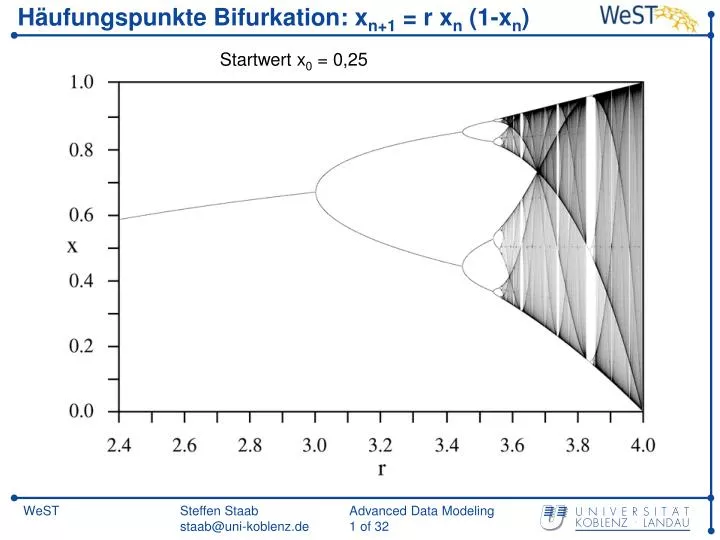
Häufungspunkte Bifurkation: x n+1 = r x n (1-x n ). Startwert x 0 = 0,25. Implementing DLV. DLV System Architecture. Rule Handling and Intelligent Grounding. Intelligent Grounding. Ground Programm has exactly the same answer sets as the original programme

E N D
Häufungspunkte Bifurkation: xn+1 = r xn (1-xn) Startwert x0 = 0,25
Intelligent Grounding • Ground Programm hasexactlythe same answersetsasthe original programme • Forsome syntactically restricted classes of programs (e.g. stratified programs), the “Intelligent Grounding” module already computes the corresponding answer sets. • We assume “safe programmes”, i.e. no variables in the head that are not bound by positive literals in the body. • We assume function-free programmes here. Thomas Eiter, Nicola Leone, Cristinel Mateis, Gerald Pfeifer, FranceseoScarcello. A Deductive System for Non-Monotonic Reasoning. In: LogicProgrammingAndNonmonotonicReasoning. Lecture Notes in Computer Science, 1997, Volume 1265/1997, 363-374, Springer.
Rules and Graphs Handler • Motivation: Overall problem of EDLP is co-NP hard, BUT many of its parts are much easier (e.g. stratified programms are polynomially computable)
Ground Dependency Graph (GG) • Nodes: atoms Edges: E+, E-, E • Ground Programme: p(2,3) :- t(2) :- q(1) q(3) :- p(2,3), NOT t(2). t(3) :- q(3), p(2,3).
Ground Collapsed Positive Dependency Graph (GG+) • Strongly connected components form modules and become one node (not in the example here)
Summarizing Steps for Analyzing Rules • Givenprogramme P, itcomputesG+ P forthe intelligent groundingmodule (IGM) • Given from IGM itcomputes GG • From and GG itsets apart • themodules, • syntacticalproperties (e.g. stratification) forthe Model Generator • ItcomputesGG+for Model Checkertoreducesearchspace • ForeachcomponentofGG+itanalyzessyntacticalproperties (e.g. headcycle-freeness) foruseby Model Checker
Grounding Init NF = EDBP % Groundedfactsinitially= DB extension = % Growgroundedprogramfrom G+P % Analyzethecollapsedngrulegraph Key stepsofprocedure: • Growrulegroundingfromnode C in G+P withoutincomingedges (i.e. non-recursive) • Growrulegroundingusing positive literals (andremovethemfromthegroundedrules!)
Example Programme Programme P p(1,2) p(2,3) :- t(X) :- a(X). q(X) q(Z) :- p(X,Y), p(Y,Z), NOT t(Y). t(X) :- q(X), p(Y,X) a(2) :- Grounded Programme p(1,2) p(2,3) :- t(2) :- q(1) q(3) :- p(1,2), p(2,3), NOT t(2). t(3) :- q(3), p(2,3) a(2) :- Note: ground(P) contains 40 rule instances, but Instantiate generates only 4.
Theorem • Let P be a safe disjunctive datalog program, and be the ground program generated by Instantiat(P). Then, P and have the same stable models.
Summary Grounding is a bit like forward chaining (applying immediate consequence operator). However, because of disjunction in the heads it is overgenerating and it is also not retracting implications that fail because of negation.
Model Generator • Derive what is definitely derivable, • Make ‘educated’ guess for one of those literals which have not been decided yet. • IF further guesses can be madeTHEN GOTO 2ELSE Call MODEL-CHECKER If candidate model is inconsistent or not stable then backtrack, taking knowledge about previous guesses into account to avoid redundancies Nicola Leone, Pasquale Rullo, Francesco Scarcello. Disjunctive Stable Models: Unfounded Sets, Fixpoint Semantics, and Computation. In: Information and Computation, 135(2): 69-112, 1997.
Note • The number of candidate models can be exponential • Smart generation of candidate models is crucial • Prune the search space! • Special algorithms for: • Polynomial-time algorithm for normal stratified programs • Special algorithm for headcycle-free disjunctive programs • General algorithm
Unfounded Sets Intuitively • An unfoundedsetfor a disjunctiveprogram P w.r.t. an interpretation I is a setof positive literalsthatcannotbederivedfrom P assumingthefacts in I. [generalizationof a techniquefrom well-foundedsemantics!]
Unfounded Sets Formally: • Let I be an interpretation for a program P. A set X of ground atoms is an unfounded set for P w.r.t. I if, for each a∈X, for each rule r∈ground(P) such that a∈H(r), at least one of the following conditions holds: • B(r) ∩ .I ≠ , that is, the body of r is false w.r.t. I • B+(r)∩ X ≠ , that is, some positive body literal belongs to X • (H(r)-X) ∩ I ≠ , that is, an atom in the head of r, distinct from a and other elements in X, is true w.r.t. I [generalization of a technique from well-founded semantics!]
Unfounded Sets: Example Program P: a b :- I = {b} Then {a} is an unfounded set of P wrt I (criterion 3 applies) Intuitively: there is no reason to believe that a is true given I
Unfounded Sets: Example Program P: a b :- I = {a,b} Then both {a} and {b} are unfounded sets of P wrt I (i.e. we should not believe both!) However, {a,b} is not an unfounded set!
Unfounded Sets: Example Program P: a b :- a :- b. b :- a. I = {a,b} Then is the only unfounded set of P wrt I
Definition & Proposition Definition • Let I be an interpretation for a program P. • I is unfounded-free if I ∩ X = for each unfounded set X for P w.r.t. I. Proposition: Let I be an unfounded-free interpretation for a program P. Then • P has the greatest unfounded set GUSP(I) • GUSP(I) is computable in polynomial time
Monotonic Operator WP Plan: • Compute WP() • Eitherthisis a uniquestablemodel • Otherwisemovefrom WP() towardsthestablemodels
Immediate Consequence Operator TP Definition: • TP(I) = {a∈BP | ∃ r∈ground(P) s.t. a∈H(r), H(r) – {a} ⊆.I, and B(r) ⊆I} Note: TP is deterministic! Definition: • WP (I) = TP(I) .GUSP(I)
Theorem Theorem • Let M be a total interpretationforprogram P. M is a stablemodelfor P iff M is a fixpointof WP. Proposition: • Given a propositional program P, WP() iscomputable in polynomial time.
Examples Program P: a b :- WP() = , i.e. not a model! Program P: b :- NOT c. a b :- WP() = {NOT c, b, NOT a}, i.e. total, i.e. stable model
Computing the Stable Models: Main Possiblytrueliterals
This slide deck is not part of the material for examinations Finis