Download
1 / 31
310 likes | 326 Vues
This research paper presents the S3P framework for self-optimizing signal processing applications to any hardware architecture. It combines system expertise and the FFTW approach to achieve optimal resource allocation.

E N D
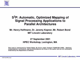
S3P: Automatic, Optimized Mapping ofSignal Processing Applications toParallel Architectures Mr. Henry Hoffmann, Dr. Jeremy Kepner, Mr. Robert Bond MIT Lincoln Laboratory 27 September 2001 HPEC Workshop, Lexington, MA This work is sponsored by United States Air Force under Contract F19628-00-C-0002. Opinions, interpretations, conclusions, and recommendations are those of the author and are not necessarily endorsed by the Department of Defense.
Acknowldegements • Matteo Frigo (MIT/LCS & Vanu, Inc.) • Charles Leiserson (MIT/LCS) • Adam Wierman (CMU)
Problem Statement • S3P Program Outline • Introduction • Design • Demonstration • Results • Summary
Beamform Latency = 2/N Filter Latency = 1/N System Latency Component Latency Local Optimum Hardware < 32 Beamform Hardware Global Optimum Latency Hardware < 32 Latency < 8 Beamform Latency < 8 Filter Filter Hardware Hardware Units (N) Example: Optimum System Latency • Simple two component system • Local optimum fails to satisfy global constraints • Need system view to find global optimum
System Optimization Challenge Signal Processing Application Beamform XOUT = w *XIN Filter XOUT = FIR(XIN) Detect XOUT = |XIN|>c Optimal Resource Allocation (Latency, Throughput, Memory, Bandwidth …) Compute Fabric (Cluster, FPGA, SOC …) • Optimizing to system constraints requires two way component/system knowledge exchange • Need a framework to mediate exchange and perform system level optimization
S3P Lincoln Internal R&D Program • Goal: applications that self-optimize to any hardware • Combine LL system expertise and LCS FFTW approach Parallel Signal Processing Kepner/Hoffmann (Lincoln) S3P Framework Algorithm Stages N 2 Processor Mappings 1 . . . S3P brings self-optimizing (FFTW) approach to parallel signal processing systems 1 2 Best Mappings Time & Verify . . . M Self-Optimizing Software Leiserson/Frigo (MIT LCS) • Framework exploits graph theory abstraction • Broadly applicable to system optimization problems • Defines clear component and system requirements
Requirements • Graph Theory Outline • Introduction • Design • Demonstration • Results • Summary
System Requirements Decomposable into Tasks (comp) and Conduits (comm) Beamform XOUT = w *XIN Filter XOUT = FIR(XIN) Detect XOUT = |XIN|>c Mappable to different sets of hardware Measurable resource usage of each mapping • Each compute stage can be mapped to different sets of hardware and timed
System Graph Beamform Filter Detect Edge is a conduit between a pair of task mappings Node is a unique mapping of a task • System Graph can store the hardware resource usage of every possible Task & Conduit
Path = System Mapping Beamform Filter Detect “Best” Path is the optimal system mapping Each path is a complete system mapping • Graph construct is very general and widely used for optimization problems • Many efficient techniques for choosing “best” path (under constraints), such as Dynamic Programming
4.0 4.0 3.0 3.0 2.0 3.0 1.0 4.0 4.0 3.0 3.0 2.0 3.0 4.0 1.0 4.0 3.0 3.0 2.0 2.0 1.0 33 23 Example: Maximize Throughput Beamform Filter Detect Edge stores conduit time for a given pair of mappings 1.5 2.0 3.0 Node stores task time for a each mapping 3.0 4.0 6.0 6.0 8.0 More Hardware 16.0 • Goal: Maximize throughput and minimize hardware • Choose path with the smallest bottleneck that satisfies hardware constraint
Path Finding Algorithms • Graph construct is very general • Widely used for optimization problems • Many efficient techniques for choosing “best” path (under constraints) such as Dikkstra’s Algorithm and Dynamic Programming N = total hardware units M = number of tasks Pi = number of mappings for task i t = M pathTable[M][N] = all infinite weight paths for( j:1..M ){ for( k:1..Pj ){ for( i:j+1..N-t+1){ if( i-size[k] >= j ){ if( j > 1 ){ w = weight[pathTable[j-1][i-size[k]]] + weight[k] + weight[edge[last[pathTable[j-1][i-size[k]]],k] p = addVertex[pathTable[j-1][i-size[k]], k] }else{ w = weight[k] p = makePath[k] } if( weight[pathTable[j][i]] > w ){ pathTable[j][i] = p } } } } t = t - 1 } Initialize Graph G Initialize source vertex s Store all vertices of G in a minimum priority queue Q while (Q is not empty) u = pop[Q] for (each vertex v, adjacent to u) w = u.totalPathWeight() + weight of edge <u,v> + v.weight() if(v.totalPathWeight() > w) v.totalPathWeight() = w v.predecessor() = u Dynamic Programming Dijkstra’s Algorithm
Required Optional S3P Inputs and Outputs Application Algorithm Information S3P Framework “Best” System Mapping System Constraints • Can flexibly add information about • Application • Algorithm • System • Hardware Hardware Information
Application • Middleware • Hardware • S3P Outline • Introduction • Design • Demonstration • Results • Summary
Middleware (PVL) Task Conduit Map S3P Engine Input Low Pass Filter Beamform Matched Filter S3P Demonstration Testbed Multi-Stage Application Hardware (Workstation Cluster)
Input Matched Filter Beamform Low Pass Filter XIN XOUT XIN XIN XOUT FFT XIN mult FIR1 FIR2 XOUT IFFT W4 W3 W1 W2 Multi-Stage Application • Features • “Generic” radar/sonar signal processing chain • Utilizes key kernels (FIR, matrix multiply, FFT and corner turn) • Scalable to any problem size (fully parameterize algorithm) • Self validates (built-in target generator)
Class Description Parallelism Matrix/Vector Used to perform matrix/vector algebra on data spanning multiple processors Data Computation Performs signal/image processing functions on matrices/vectors (e.g. FFT, FIR, QR) Data & Task Signal Processing & Control Task Supports algorithm decomposition (i.e. the boxes in a signal flow diagram) Task & Pipeline Conduit Supports data movement between tasks (i.e. the arrows on a signal flow diagram) Task & Pipeline Map Specifies how Tasks, Matrices/Vectors, and Computations are distributed on processor Data, Task & Pipeline Mapping Grid Organizes processors into a 2D layout Parallel Vector Library (PVL) • Simple mappable components support data, task and pipeline parallelism
Hardware Platform • Network of 8 Linux workstations • Dual 800 MHz Pentium III processors • Communication • Gigabit ethernet, 8-port switch • Isolated network • Software • Linux kernel release 2.2.14 • GNU C++ Compiler • MPICH communication library over TCP/IP • Advantages • Software tools • Widely available • Inexpensive (high Mflops/$) • Excellent rapid prototyping platform • Disadvantages • Non real-time OS • Non real-time messaging • Slower interconnect • Difficulty to model • SMP behavior erratic
S3P Engine Application Program Algorithm Information “Best” System Mapping S3P Engine System Constraints Hardware Information MapGenerator MapTimer MapSelector • Map Generator constructs the system graph for all candidate mappings • Map Timer times each node and edge of the system graph • Map Selector searches the system graph for the optimal set of maps
Simulated/Predicted/Measured • Optimal Mappings • Validation and Verification Outline • Introduction • Design • Demonstration • Results • Summary
8.3 12 52 8.7 49 31 3.3 46 - 2.6 42 57 7.3 16 47 8.3 17 27 9.4 21 - 8.0 28 24 44 14 - 9.1 29 - 20 - - 18 24 - Input Low Pass Filter Matched Filter Beamform 18 60 17 15 33 14 23 14 - 14 15 13 3.2 31.5 16.1 31.4 Best 30 msec (1.6 MHz BW) 1.4 15.7 9.8 18.0 Best 15 msec (3.2 MHz BW) 1.0 10.4 6.5 13.7 0.7 8.2 3.3 11.5 Optimal Throughput • Vary number of processors used on each stage • Time each computation stage and communication conduit • Find path with minimum bottleneck 1 CPU 2 CPU 3 CPU 4 CPU
Input Low Pass Filter Beamform Matched Filter S3P Timings (4 cpu max) • Graphical depiction of timings (wider is better) 4 CPU 3 CPU 2 CPU 1 CPU Tasks
S3P Timings (12 cpu max)(wider is better) 12 CPU 8 CPU 6 CPU 4 CPU 2 CPU • Large amount of data requires algorithm to find best path Input Low Pass Filter Beamform Matched Filter Tasks
Predicted and Achieved Latency(4-8 cpu max) Large (48x128K) Problem Size Small (48x4K) Problem Size Latency (sec) Latency (sec) Maximum Number of Processors Maximum Number of Processors • Find path that produces minimum latency for a given number of processors • Excellent agreement between S3P predicted and achieved latencies
Predicted and Achieved Throughput(4-8 cpu max) Large (48x128K) Problem Size Small (48x4K) Problem Size Throughput (pulses/sec) Throughput (pulse/sec) Maximum Number of Processors Maximum Number of Processors • Find path that produces maximum throughput for a given number of processors • Excellent agreement between S3P predicted and achieved throughput
SMP Results (16 cpu max) Large (48x128K) Problem Size Throughput (pulse/sec) Maximum Number of Processors • SMP overstresses Linux Real Time capabilities • Poor overall system performance • Divergence between predicted and measured
Simulated (128 cpu max) Small (48x4K) Problem Size Small (48x4K) Problem Size Throughput (pulses/sec) Latency (sec) Maximum Number of Processors Maximum Number of Processors • Simulator allows exploration of larger systems
Reducing the Search Space-Algorithm Comparison- Graph algorithms provide baseline performance Hill Climbing performance varies as a function of initialization and neighborhood definition Number of Timings Required Preprocessor outperforms all other algorithms. Maximum Number of Processors
Future Work • Program area • Determine how to enable global optimization in other middleware efforts (e.g. PCA, HPEC-SI, …) • Hardware area • Scale and demonstrate on larger/real-time system • HPCMO Mercury system at WPAFB • Expect even better results than on Linux cluster • Apply to parallel hardware • MIT/LCS RAW • Algorithm area • Exploits ways of reducing search space • Provide solution “families” via sensitivity analysis
Outline • Introduction • Design • Demonstration • Results • Summary
Summary • System level constraints (latency, throughput, hardware size, …) necessitate system level optimization • Application requirements for system level optimization are • Decomposable into components (input, filtering, output, …) • Mappable to different configurations (# processors, # links, …) • Measureable resource usage (time, memory, …) • S3P demonstrates global optimization is feasible separate from the application