Download
1 / 27
280 likes | 456 Vues
Chapter 6 Random Processes. Description of Random Processes Stationarity and ergodicty Autocorrelation of Random Processes Properties of autocorrelation. Huseyin Bilgekul EEE 461 Communication Systems II Department of Electrical and Electronic Engineering Eastern Mediterranean University.

E N D
Chapter 6Random Processes • Description of Random Processes • Stationarity and ergodicty • Autocorrelation of Random Processes • Properties of autocorrelation Huseyin Bilgekul EEE 461 Communication Systems II Department of Electrical and Electronic Engineering Eastern Mediterranean University
Homework Assignments • Return date: November 8, 2005. • Assignments: Problem 6-2 Problem 6-3 Problem 6-6 Problem 6-10 Problem 6-11
Random Processes • A RANDOM VARIABLEX, is a rule for assigning to every outcome, w, of an experiment a number X(w). • Note: X denotes a random variable and X(w) denotes a particular value. • A RANDOM PROCESSX(t) is a rule for assigning to every w, a function X(t,w). • Note: for notational simplicity we often omit the dependence on w.
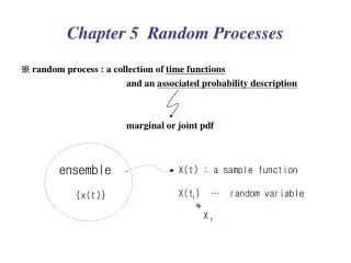
Ensemble of Sample Functions The set of all possible functions is called the ENSEMBLE.
Random Processes • A general Random or Stochastic Process can be described as: • Collection of time functions (signals) corresponding to various outcomes of random experiments. • Collection of random variables observed at different times. • Examples of random processes in communications: • Channel noise, • Information generated by a source, • Interference. t1 t2
Collection of Time Functions • Consider the time-varying function representing a random process where wi represents an outcome of a random event. • Example: • a box has infinitely many resistors (i=1,2, . . .) of same resistance R. • Let wi be event that the ith resistor has been picked up from the box • Let v(t, wi) represent the voltage of the thermal noise measured on this resistor.
Collection of Random Variables • For a particular time t=to the value x(to,wi) is a random variable. • To describe a random process we can use collection of random variables {x(to,w1) , x(to,w2) , x(to,w3) , . . . }. • Type: a random processes can be either discrete-time or continuous-time. • Probability of obtaining a sample function of a RP that passes through the following set of windows. Probability of a joint event.
Description of Random Processes • Analytical description:X(t) =f(t,w) where w is an outcome of a random event. • Statistical description: For any integer N and any choice of (t1, t2, . . ., tN) the joint pdf of {X(t1), X( t2), . . ., X( tN) } is known. To describe the random process completely the PDF f(x) is required.
Example: Analytical Description • Let where q is a random variable uniformly distributed on [0,2p]. • Complete statistical description of X(to)is: • Introduce • Then, we need to transform from y to x: • We need both y1 and y2 because for a given x the equation x=A cos(y) has two solutions in [0,2p].
Analytical (continued) • Note x and y are actual values of the random variables X and Y. • Since and pY is uniform in [2pf0t0, 2pf0t0 + 2p], we get • Using the analytical description of X(t),we obtained its statistical description at any time t.
Example: Statistical Description • Suppose a random process x(t) has the property that for any N and (t0,t1, . . .,tN) the joint density function of {x(ti)}is a jointly distributed Gaussian vector with zero mean and covariance • This gives complete statistical description of the random process x(t).
x(t) x(t) 2 B t t B intersect is Random Activity: Ensembles • Consider the random process: x(t)=At+B • Draw ensembles of the waveforms: • B is constant, A is uniformly distributed between [-1,1] • A is constant, B is uniformly distributed between [0,2] • Does having an “Ensemble” of waveforms give you a better picture of how the system performs? Slope Random
Stationarity • Definition: A random process is STATIONARY to the order N if for any t1,t2, . . . , tN, fx{x(t1), x(t2),...x(tN)}=fx{x(t1+t0), x(t2+t0),...,x(tN +t0)} • This means that the process behaves similarly (follows the same PDF) regardless of when you measure it. • A random process is said to be STRICTLY STATIONARY if it is stationary to the order of N→∞. • Is the random process from the coin tossing experiment stationary?
Illustration of Stationarity Time functions pass through the corresponding windows at different times with the same probability.
Example of First-Order Stationarity • Assume that A and w0 are constants; q0 is a uniformly distributed RV from [-p,p);t is time. • From last lecture, recall that the PDF of x(t): • Note: there is NO dependence on time, the PDF is not a function of t. • The RP is STATIONARY.
Non-Stationary Example • Now assume that A,q0 and w0 are constants; t is time. • Value of x(t) is always known for any time with a probability of 1. Thus the first order PDF of x(t) is • Note: The PDF depends on time, so it is NONSTATIONARY.
Ergodic Processes • Definition: A random process is ERGODIC if all time averages of any sample function are equal to the corresponding ensemble averages (expectations) • Example, for ergodic processes, can use ensemble statistics to compute DC values and RMS values • Ergodic processes are always stationary; Stationary processes are not necessarily ergodic
Example: Ergodic Process • A and w0 are constants; q0 is a uniformly distributed RV from [-p,p);t is time. • Mean (Ensemble statistics) • Variance
Example: Ergodic Process • Mean (Time Average) T is large • Variance • The ensemble and time averages are the same, so the process is ERGODIC
EXERCISE • Write down the definition of : • Wide sense stationary • Ergodic processes • How do these concepts relate to each other? • Consider: x(t) = K; K is uniformly distributed between [-1, 1] • WSS? • Ergodic?
Autocorrelation of Random Process • The Autocorrelation function of a real random process x(t) at two times is:
Wide-sense Stationary • A random process that is stationary to order 2 or greater is Wide-Sense Stationary: • A random process is Wide-Sense Stationaryif: • Usually, t1=t and t2=t+tso that t2- t1 =t. • Wide-sense stationary process does not DRIFT with time. • Autocorrelation depends only on the time gap but not where the time difference is. • Autocorrelation gives idea about the frequency response of the RP.
Autocorrelation Function of RP • Properties of the autocorrelation function of wide-sense stationary processes Autocorrelation of slowly and rapidly fluctuating random processes.
Cross Correlations of RP • Cross Correlation of two RP x(t) and y(t) is defined similarly as: • If x(t) and y(t) are Jointly Stationary processes, • If the RP’s are jointly ERGODIC,
Cross Correlation Properties of Jointly Stationary RP’s • Some properties of cross-correlation functions are • Uncorrelated: • Orthogonal: • Independent: if x(t1) and y(t2) are independent (joint distribution is product of individual distributions)