Download
1 / 51
550 likes | 854 Vues
Implementation & Computation of DW and Data Cube. Remember: ....What is OLAP?. The term OLAP („online analytical processing“) was coined in a white paper written for Arbor Software Corp. in 1993. Data Cube, Storage space Partial, total and no materialization (precomputation)

E N D
Remember: ....What is OLAP? • The term OLAP („online analytical processing“) was coined in a white paper written for Arbor Software Corp. in 1993
Data Cube, Storage space • Partial, total and no materialization (precomputation) • How to select cuboids for materialization and how to use them • Indexing • Multiway array aggregation • Constraints for the curse of dimensionality • Discovery driven explanation
Data warehouse contains huge volumes of data • OLAP servers demand that the decision support queries be answered in order of seconds • Highly efficient cube computation techniques • Access methods • Query processing techniques
Core of multidimensional data analysis is the efficient of aggregation across many sets of dimension • The compute cube operator aggregates over all subsets of dimensions
You would like to create a data cubeAll_Electronics that contains the following: • item, city, year, and sales_in_Euro • Answer following queries • Compute the sum of sales, grouping by item and city • Compute the sum of sales, grouping by item • Compute the sum of sales, grouping by city
The total number of data cuboids is 23=8 • {(city,item,year), • (city,item), (city,year), • (city),(item),(year), • ()} • (), the dimensions are not grouped • These group-by’s form a lattice of cuboids for the data cube • The basic cuboid contains all three dimensions
() (city) (item) (year) (city, item) (city, year) (item, year) (city, item, year) • Hasse-Diagram:Helmut Hasse 1898 - 1979 did fundamental work in algebra and number theory
For a cube with n dimensions, there are total 2n cuboids • A cube operator was first proposed by Gray et. All 1997: • Data Cube: A Relational Aggregation Operator Generalizing Group-By, Cross-Tab, and Sub-Totals; J. Gray, S. Chaudhuri, A. Bosworth, A. Layman, D. Reichart, M. Venkatrao, F. Pellow, H. Pirahesh: Data Mining and Knowledge Discovery 1(1), 1997, 29-53. • http://research.microsoft.com/~Gray/
On-line analytical processing may need to access different cuboids for different queries • Compute some cuboids in advance • Precomputation leads to fast response times • Most products support to some degree precomputation
Storage space may explode... • If there are no hierarchies the total number for n-dimensional cube is 2n • But.... • Many dimensions may have hierarchies, for example time • day < week < month < quarter < year • For a n-dimensional data cube, where Li is the number of all levels (for time Ltime=5), the total number of cuboids that can be generated is
It is unrealistic to precompute and materialize (store) all cuboids that can be generated • Partial materialization • Only some of possible cuboids are generated
No materialization • Do not precompute any of “nonbase” cuboids • Expensive computation in during data analysis • Full materialization • Precompute all cuboids • Huge amount of memory.... • Partial materialization • Which cuboids should we precompute and which not?
Partial materialization -Selection of cuboids • Take into account: • the queries, their frequencies, the accessing costs • workload characteristics, costs for incremental updates, storage requirements • Broad context of physical database design, generation and selection of indices
Heuristic approaches for cuboid selection • Materialize the set of cuboids on which other popular referenced cuboids are based
It is important to take advantage of materialized cuboids during query processing • How to use available index structures on the materialized cuboids • How to transform the OLAP operations into the selected cuboids
Determine which operations should be preformed on the available cuboids • This involves transforming any selection, projection, roll-up and drill down operations in the query into corresponding SQL and/or OLAP operations • Determine to which materialized cuboids the relevant operations should be applied • Identifying all materialized cuboids that may potentially by used to answer the query
Example • Suppose that we define a datacube for ALLElectronics of the form • sales[time,item,location]: sum(salles_in_euro) • Dimension hierarchies • time: day < month < quater < year • Item: item_name < brand < type
Query • {brand,province_or_state} with year=2000 • Four materialized cubes are available 1) {year, item_name, city} 2) {year, brand, country} 3) {year, brand, province_or_state} 4) {item_name, province_or_state} where year = 2000 • Which should be selected to process the query?
Finer granularity data cannot be generated from coarser-granularity data • Cuboid 2 cannot be used since country is more general concept then province_or_state • Cuboids 1, 3, 4 can be used • They have the same set or superset of the dimensions of the query • The selection clause in the query can imply the selection in the cuboid • The abstraction levels for the item and location dimension in these cuboids are at a finer level than brand and province_or_state
How would the costs of each cuboid compare? • Cuboid 1 would cost the most, since both item_name and city are at a lower level than brand and province_or_state • If not many year values associated with items in the cube, and there are several item names for each brand, then cuboid 3 will be better than cuboid 4 • Efficient indices available for cuboid 4, cuboid 4 better choice (bitmap indexes)
Indexing OLAP Data: Bitmap Index • Index on a particular column • Each value in the column has a bit vector: bit-op is fast • The length of the bit vector: # of records in the base table • The i-th bit is set if the i-th row of the base table has the value for the indexed column Base table Index on Region Index on Type
Bitmap Index • Allows quick search in data cubes • Advantageous compared to hash and tree indices • Useful for low-cardinality domains because comparison, join, and aggregation operations are reduced to bitmap arithmetic's • (Reduced processing time!) • Significant reduction in space and I/O since a string of character can be represented by a bit
Join indexing method • The join indexing method gained popularity from its use in relational database query processing • Traditional indexing maps the value in a given column to a list of rows having that value • For example, if two relations R(RID,A) and S(B,SID) join on two attributes A and B, then the join index record contains the pair (RID,SID) from R and S relation • Join index records can identify joinable tuples without performing costly join operators
Indexing OLAP Data: Join Indices In data warehouses, join index relates the values of the dimensions of a start schema to rows in the fact table. • E.g. fact table: Sales and two dimensions city and product • A join index on city maintains for each distinct city a list of R-IDs of the tuples recording the Sales in the city • Join indices can span multiple dimensions
Multiway Array Aggregation • Sometimes we need to precompute all of the cuboids for a given data cube • (full materialization) • Cuboids can be stored on secondary storage and accessed when necessary • Methods must take into account the limited amount of main memory and time • Different techniques for ROLAP and MOLAP
Partitioning • Usually, entire data set can’t fit in main memory • Sort distinct values, partition into blocks that fit • Continue processing • Optimizations • Partitioning • External Sorting, Hashing, Counting Sort • Ordering dimensions to encourage pruning • Cardinality, Skew, Correlation • Collapsing duplicates • Can’t do holistic aggregates anymore!
ROLAP cube computation • Sorting hashing and grouping operations are applied to the dimension attributes in order to reorder and group related tuples • Grouping is preformed on some sub aggregates as a partial grouping step • Speed up computation • Aggregate may be computed from previously computed aggregates, rather than from the base fact tables
MOLAB and cube computation • MOLAP cannot perform the value-based reordering because it uses direct array addressing • Partition arrays into chunks (a small subcube which fits in memory). • Compressed sparse array addressing for empty cell arrays • Compute aggregates in “multiway” by visiting cube cells in the order which minimizes the number of times to visit each cell, and reduces memory access and storage cost
Example 3-D data array containing the dimensions A,B,C • Array is partitioned into small, memory based chunks • Array is partitioned into 64 chunks • Full materialization • The base cuboid denoted by ABC from which all other cuboids are directly computed. This cuboid is already computed • The 2-D cuboids AB, AC, BC (has to be computed) • The 1-D cuboid A, B, C (has to be computed) • 0-D (ppax) must be also computed
C c3 61 62 63 64 c2 45 46 47 48 c1 29 30 31 32 c 0 B 60 13 14 15 16 b3 44 28 56 9 b2 B 40 24 52 5 b1 36 20 1 2 3 4 b0 a0 a1 a2 a3 A What is the best traversing order to do multi-way aggregation?
Suppose we would like to compute the b0c0 chunk of the BC cuboid • We allocate space for this chunk in the chunk memory • By scanning chunks 1 to 4 of the b0c0 chunk is computed • The chunk memory can be assigned to the next chunks • BC cuboid can be computed using only one chunk of memory!
C c3 61 62 63 64 c2 45 46 47 48 c1 29 30 31 32 c 0 B 60 13 14 15 16 b3 44 28 56 9 b2 40 24 52 5 b1 36 20 1 2 3 4 b0 a0 a1 a2 a3 A Multi-way Array Aggregation for Cube Computation B
Multiway of computation • When chunk 1 is being scanned, all other 2-D chunks relating to the chunk 1can be simultaneously be computed
Example • Suppose the size of the array for each dimension A,B,C is 40,400,4000 • The size of each partition is therfore 10,100,1000 • Size of BC is 400*4000=1.600.000 • Size of AC is 40*4000=1.60.000 • Size of AB is 40*400=16.000
Scanning in the order 1 to 64 • Aggregation of chunk bycz requires scanning 4 chunks • Aggregation of chunk axcz requires scanning 13 chunks • Aggregation of chunk axby requires scanning 49 chunks
Multi-way Array Aggregation for Cube Computation C c3 61 62 63 64 c2 45 46 47 48 c1 29 30 31 32 c 0 B 60 13 14 15 16 b3 44 28 B 56 9 b2 40 24 52 5 b1 36 20 1 2 3 4 b0 a0 a1 a2 a3 A
To aoid bringing 3-D chunk into memory more than once • Ordering 1-64: • One for chunk of the BC plane 100*1000 • For one row of the AC plane 10*4000 • For the whole AB plane 40*400 • + -------------------- • =156.000
Suppose, scanned in differend order, first agregation towards the smallest AB plane, and than towards the AC plane: • One for chunk of the AB plane 400*4000 • For one row of the AC plane 10*4000 • For the whole BC plane 10*100 • + -------------------- • =1.641.000 • 10 times more moemory
Multi-Way Array Aggregation for Cube Computation • Method: the planes should be sorted and computed according to their size in ascending order • Idea: keep the smallest plane in the main memory, fetch and compute only one chunk at a time for the largest plane • Limitation of the method: computing well only for a small number of dimensions • The number of the cuboids is exponential to the number of dimensions (2N)
Overcome the curse of dimensionality • Use constrains, for example “iceberg cube” • Compute only those combinations of attribute values that satisfy a minimum support requirement or other aggregate condition, such as average, min, max, or sum • The term "iceberg" was selected because these queries retrieve a relatively small amount of the data in the cube, i.e. the "tip of the iceberg”
Iceberg Cube • Computing only the cuboid cells whose count or other aggregates satisfying the condition like HAVING COUNT(*) >= minsup • Motivation • Only calculate “interesting” cells—data above certain threshold • Avoid explosive growth of the cube • Suppose 100 dimensions, only 1 base cell. How many aggregate cells if count >= 1? What about count >= 2?
BUC (Bottom-Up Computation) • This algorithm computes the cube beginning with the smallest, most aggregated cuboid and recursively works up to the largest, least aggregated cuboids. • If the cuboid does not satisfy the minimum support condition, then the algorithm does not calculate the next largest cuboid
Discovery driven Exploration • A user analyst search for interesting patterns in the cube by the operations • User following his one hypothesis and knowledge tries to recognize exceptions or anomalies • Problems: • Search space very large • Solution: • Indicate data exceptions automatically
Exception • Data value which significantly different, based on statistical model • Residual value • Scale values based on the standard deviation • If the scaled value exceeds a specified threshold
Kinds of Exceptions and their Computation • Parameters • SelfExp: surprise of cell relative to other cells at same level of aggregation • InExp: surprise beneath the cell (less aggregate, finer resolution) • PathExp: surprise beneath cell for each drill-down path • Computation of exception indicator (modeling fitting and computing SelfExp, InExp, and PathExp values) can be overlapped with cube construction • Exception themselves can be stored, indexed and retrieved like precomputed aggregates
Discovery-Driven Data Cubes SelExp InExp
Data Cube, Storage space • Partial, total and no materialization (precomputation) • How to select cuboids for materialization and how to use them • Indexing • Multiway array aggregation • Constraints for the curse of dimensionality • Discovery driven explanation
Design of DW • DMQL, MDX