Download
1 / 26
260 likes | 470 Vues
Outline. terminating and non-terminating systems analysis of terminating systems generation of random numbers simulation by Excel a terminating system a non-terminating system basic operations in Arena. Two Types of Systems Terminating and Non-Terminating. chess piece

E N D
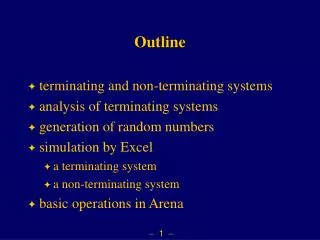
Outline • terminating and non-terminating systems • analysis of terminating systems • generation of random numbers • simulation by Excel • a terminating system • a non-terminating system • basic operations in Arena
chess piece starts at vertex F moves equally likely to adjacent vertices to estimate E(# of moves) to reach the upper boundary GI/G/ 1 queue infinite buffer service times ~ unif[6, 10] interarrival times ~ unif[8, 12] to estimate the E[# of customers in system] N(t) … t, time B A C D E F Two Types of Systems
chess piece initial condition defined by problem termination of a simulation run defined by the system estimation of the mean or probability of a random variable run length defined by number of replications GI/G/ 1 queue initial condition unclear termination of a simulation run defined by ourselves estimation of the mean or probability of the limit of a sequence of random variables run length defined by run time Two Types of Systems
chess piece: a terminating systems analysis: Strong Law of Large Numbers (SLLN) and Central Limit Theorem (CLT) GI/G/ 1 queue: a non-terminating system analysis: probability theory and statistics related to but not exactly SLLN, nor CLT Two Types of Systems Terminating and Non-Terminating
define Strong Law of Large Numbers - Basis to Analyze Terminating Systems • i.i.d. random variables X1, X2, … • finite mean and variance 2
What be? Strong Law of Large Numbers - Basis to Analyze Terminating Systems • a fair die thrown continuously • Xi = the number shown on the ith throw
Strong Law of Large Numbers - Basis to Analyze Terminating Systems • in terminating systems, each replication is an independent draw of X • Xiare i.i.d. • E(X) (X1 + … + Xn)/n
Central Limit Theorem - Basis to Analyze Terminating Systems • interval estimate & hypothesis testing of normal random variables • t, 2, and F • i.i.d. random variables X1, X2, … of finite mean and variance 2 • CLT: approximately normal for “large enough”n • can use t, 2, and Ffor
To Generate Random Variates in Excel • for uniform [0, 1]:rand() function • for other distributions: use Random Number Generator in Data Analysis Tools • uniform, discrete, Poisson, Bernoulli, Binomial, Normal • tricks to transform • uniform [-3.5, 7.6]? • normal (4, 9)(where 4 is the mean and 9 is the variance)?
To Generate the Random Mechanism • general overview, with details discussed later this semester • everything based on random variates from uniform (0, 1) • each stream of uniform (0, 1) random variates being a deterministicsequence of numbers on a round robin • “first” number in the robin to use: SEED • many simple, handy generators
Examples • Example 1: Generate 1000 samples of X~ uniform(0,1) • Example 2: Generate 1000 samples of Y ~ normal(5,1) • Example 3: Generate 1000 samples of Z ~ z: 5 10 15 20 25 30 p: 0.1 0.15 0.3 0.2 0.14 0.11 • Example 4. Use simulation to estimate (a) P(X > 0.5) (b) P(2 < Y < 8) (c) E(Z) Using 10 replications, 50 replications, 500 replications, 5000 replications. Which is more accurate?
Y = Examples: Probability and Expectation of Functions of Random Variables • X ~ x: 100 150 200 250 300 p(x): 0.1 0.3 0.3 0.2 0.1 • Find E(Y) and P(Y 30)
Examples: Probability and Expectation of Functions of Random Variables • X ~ N(10, 4),Y ~ N(9,1), independent • estimate • P(X < Y) • Cov(X, Y) = E(XY) - E(X)E(Y)
Example: Newsboy Problem Pieces of “Newspapers” to Order • order 2012 calendars in Sept 2011 • cost: $2 each; selling price: $4.50 each • salvage value of unsold items at Jan 1 2012: $0.75 each • from historical data: demand for new calendars Demand: 100 150 200 250 300 Prob. : 0.3 0.2 0.3 0.15 0.05 • objective: profit maximization • questions • how many calendars to order • with the optimal order quantity, P(profit 400)
Example: Newsboy Problem Pieces of “Newspapers” to Order • D = the demand of the 2012 calendar • D follows the given distribution • Q = the order quantity {100, 150, 200, 250, 300} • V = the profit in ordering Q pieces • = 4.5 min (Q, D) + 0.75 max (0, Q - D) - 2Q • objective: find Q* to maximize E(V)
Example: Newsboy Problem Pieces of “Newspapers” to Order • two-step solution procedure • 1 estimate E(profit) for a given Q • generate demands • find the profit for each demand sample • find the (sample) mean profit of all demand samples • 2 look for Q*, which gives the largest mean profit
Example: Newsboy Problem Pieces of “Newspapers” to Order • our simulation of 1000 samples, • Q = 100: E(V) = 250 • Q = 150: E(V) = 316.31 • Q = 200: E(V) = 348.31 • Q = 250: E(V) = 328.75 • Q = 300: E(V) = 277.17 • Q* = 200 is optimal • remarks: many papers on this issue
Simulation a GI/G/1 Queue by its Special Properties • Dn = delay time of the nth customer; D1 = 0 • Sn = service time of the nth customer • Tn = inter-arrival time between the nst and the (n+1)st customer • Dn+1 = [Dn + Sn - Tn]+, where []+ = max(, 0) • average delay =
a drill press Model 03-01 • a drill press processing one type of product • interarrival times ~ i.i.d. exp(5) • service times ~ i.i.d. triangular (1,3,6) • all random quantities are independent one type of parts; parts come in and are processed one by one
Model 03-02 and Model 03-03 • Model 03-02: sequential servers • Alfie checks credit • Betty prepares covenant • Chuck prices loan • Doris disburses funds • Model 03-03: parallel servers • Each employee can do any tasks


