Download
1 / 8
80 likes | 226 Vues
Structure of Heavy Precipitation Over California Mei Han, Code 612, NASA/GSFC and Morgan State University/GESTAR Scott A. Braun, Code 612, NASA/GSFC; Toshihisa Matsui, Code 612, NASA/GSFC and UMD/ESSIC.

E N D
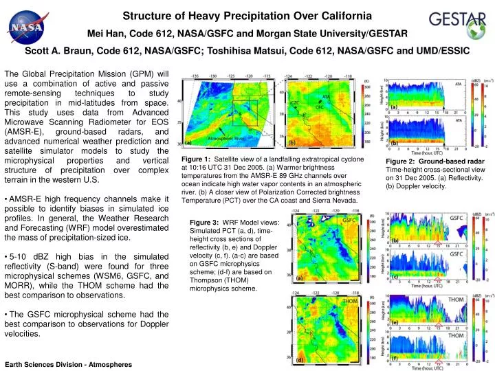
Structure of Heavy Precipitation Over California Mei Han, Code 612, NASA/GSFC and Morgan State University/GESTAR Scott A. Braun, Code 612, NASA/GSFC; Toshihisa Matsui, Code 612, NASA/GSFC and UMD/ESSIC • The Global Precipitation Mission (GPM) will use a combination of active and passive remote-sensing techniques to study precipitation in mid-latitudes from space. This study uses data from Advanced Microwave Scanning Radiometer for EOS (AMSR-E), ground-based radars, and advanced numerical weather prediction and satellite simulator models to study the microphysical properties and vertical structure of precipitation over complex terrain in the western U.S. • AMSR-E high frequency channels make it possible to identify biases in simulated ice profiles. In general, the Weather Research and Forecasting (WRF) model overestimated the mass of precipitation-sized ice. • 5-10 dBZ high bias in the simulated reflectivity (S-band) were found for three microphysical schemes (WSM6, GSFC, and MORR), while the THOM scheme had the best comparison to observations. • The GSFC microphysical scheme had the best comparison to observations for Doppler velocities. Figure 1:Satelliteview of a landfalling extratropical cyclone at 10:16 UTC 31 Dec 2005. (a) Warmer brightness temperatures from the AMSR-E 89 GHz channels over ocean indicate high water vaporcontents in an atmospheric river. (b) A closer view of Polarization Corrected brightness Temperature (PCT) over the CA coast and Sierra Nevada. Figure 2:Ground-based radar Time-height cross-sectional view on 31 Dec 2005. (a) Reflectivity. (b) Doppler velocity. Figure 3: WRF Model views: Simulated PCT (a, d), time-height cross sections of reflectivity (b, e) and Doppler velocity (c, f). (a-c) are based on GSFC microphysics scheme; (d-f) are based on Thompson (THOM) microphysics scheme. Earth Sciences Division - Atmospheres
Name: Mei Han, NASA/GSFC, Code 612 and Morgan State University/GESTAR E-mail: mei.han-1@nasa.gov Phone: 301-614-6336 References: Han, M., S. A. Braun, T. Matsui, and C. R. Williams (2013), Evaluation of cloud microphysics schemes in simulations of a winter storm using radar and radiometer measurements. Journal of Geophysical Research: Atmospheres, 118, 1401-1419. Data Sources: NASA AQUA AMSR-E (brightness temperature) NOAA HMT SPROF (radar reflectivity and Doppler velocity) Technical Description of Figures: Figure 1: Panel (a) shows brightness temperature obtained from the 89 GHz channels of the AMSR-E radiometer during one overpass. The warm colors (yellow to orange) over the East Pacific depicts the emission from the high water vapor content associated with the atmospheric river. The term “atmospheric river” refers to the route of abundant moisture transported onshore by the pre-frontal low-level jet in the extratropical cyclone’s warm sector. In panel (b), the Polarization Corrected Temperature (PCT) is used to characterize the scattering of high frequency microwaves (≥ 35 GHz) by ice hydrometeors and to contrast the low emission from the cold ocean background. Figure 2: Time-height cross section of (a) reflectivity and (b) Doppler velocity obtained by a S-band profiling radar (S-PROF) at Alta, CA (i.e. ATA, 1085 m MSL). Three S-PROF radars were deployed by the NOAA Hydrometeorology Testbed (HMT) program. See crosses in Fig. 1b for their locations. In panel (a), the greatest reflectivity occurring at ~2.5 km indicating the melting level. Above that level, the relatively weak reflectivity (< 30 dBZ) indicates a snow layer with rain below. Doppler velocities (b) show slow and fast fall velocities associated with snow and rain, respectively, and similarly indicate the location of the melting level. Black arrows indicate the time of frontal passage. Figure 3: WRF and Goddard-Satellite Data Simulator Unit (G-SDSU) simulations of PCT (a,d), reflectivity (b,e), and Doppler velocity (c,f). Two microphysics schemes, GSFC and THOM, are shown for comparison in this highlight. A general bias of ~ 20 K or larger are found in PCT, showing too much scattering that implies an overestimate of precipitating ice aloft. GSFC shows a 5 dBZ or larger bias in reflectivity magnitude for snow, while THOM agrees with observations better. In terms of the magnitudes of the Doppler velocity, GSFC agrees well with the observations in the snow layer, while THOM shows a slight high bias. The top vertex of red triangles indicates the time of front passage. Two additional schemes (WSM6 and Morrison 2-moment, i.e., MORR) are examined in Han et al. (2013).The unique snow size distribution and fractal-like shape assumptions in THOM result in a better simulation of reflectivity, while slower fall speeds in the speed-diameter relationship assumption in GSFC contribute to its good performance on the Doppler velocity simulation. Scientific significance: This research addresses a key NASA Precipitation Measurement Missions science topic, to use advanced space-borne sensors to gain physical insights into precipitation processes. Using both space-borne and ground-based observations, we investigated the impact of four widely used microphysics schemes in WRF model on precipitation scattering signature, reflectivity, and Doppler velocity. we also obtained in-depth insights regarding assumptions related to particle size distribution, shape, fall velocity, and their relationship to remote sensing quantities for the four schemes in WRF. Methodologies developed to simulate those remote sensing quantities could be contributed to a larger scientific community. Relevance for Future Missions: Our research using NASA satellites in evaluation of the performance of a sophisticated numerical weather model contributions to the NASA goal of improving weather prediction of extreme events. Earth Sciences Division - Atmospheres
Successful Forecasting of Propagating Precipitation Events by the NASA Unified-Weather Research and Forecasting Model Wei-Kuo Tao (GSFC), Di Wu(SSAI), Toshihisa Matsui (ESSIC), Stephen Lang (SSAI), Code 612, NASA GSFC • A regional high-resolution model was used to conduct a series of real-time forecasts during the Midlatitude Continental Convective Clouds Experiment (MC3E) in 2011 over the Southern Great Plains (SGP). This study utilized the model dataset to investigate one type of diurnal precipitation variation generated by eastward-propagating mesoscale convective systems (MCS) that are responsible for a majority of warm season precipitation in the central USA, from the lee side of the Rocky Mountains into the SGP. This study evaluates model simulations with regard to rainfall using observations and assesses the impact of microphysics, surface fluxes, radiation and terrain on the simulated diurnal rainfall variation. • The model ably captured most heavy precipitation events. When all forecast days are composited, the mean forecast depicts accurate, propagating precipitation features and thus the overall diurnal variation. • Post mission case studies suggest that cold-pool dynamics influences the MCSs’ organization and propagation. Terrain affects on the initial stages of MCS development. Surface and radiation processes only have a secondary effect on the diurnal variation of precipitation for short-term forecasts. Figure 1: Hourly accumulated surface rainfall from (a)-(d) observation-based NLDAS and (e)-(h) a WRF simulation with LIS. (a) and (e) are at 09 UTC, (b) and (f) 15 UTC, (c) and (g) 21 UTC 20 May and (d) and (h) are at 01 UTC 21 May 2011. NU-WRF systematically underestimates the area coverage of light precipitation. Figure 2:Time series of hourly precipitation from 00 UTC 20 May to 00 UTC 22 May 2011 from NLDAS (nldas, black) and WRF simulations with LIS (narrlis, purple), without terrain height (terr0.0, red) and without sensible and latent heat fluxes (sfx0.0, gold). Earth Sciences Division - Atmospheres
Name: Wei-Kuo Tao, NASA/GSFC, Code 612 E-mail: wei-kuo.tao-1@nasa.gov Phone: 301-614-6269 References: Tao, W.-K., D. Wu, T. Matsui, C. Peters-Lidard, S. Lang, A. Hou, M. Rienecker, W. Petersen and M. Jensen, 2013: The Diurnal Variation of Precipitation: A numerical modeling study, Journal of Geophysical Research, doi: 10.1002/jgrd.50410, (July Issue). Lang, S., W.-K. Tao, X. Zeng and Y. Li, 2011: Reducing the biases in simulated radar reflectivities from a bulk microphysics scheme: Tropical convective systems, Journal of the Atmospheric Sciences, 68, 2306-2320. Matsui, T., D. Mocko, M.-I. Lee, J. Chern and W.-K. Tao, 2010: Ten-year climatology of summertime diurnal rainfall rate over the conterminous U.S., Geophysical Research Letters, 37, L13807, doi:10.1029/2010GL044139. Data Sources: NEXRAD radar reflectivity, North American Regional Reanalysis (NARR), North American Mesoscale Model (NAM), and the North American Land Data Assimilation System (NLDAS). Some simulations used the Land Information System (LIS) land data assimilation system for surface conditions. Technical Description of Figures: Figure 1: For the 20 May case, the observations show a classic continental multi-cell squall line structure with leading convective cells and a widespread trailing stratiform region. The simulated rainfall captured the observed early (03-09 UTC 20 May), mature (09-19 UTC 20 May), and decaying stages (19 UTC 20 May-00 UTC 21 May) as well as a period of new cell development (00-06 UTC 21 May). However, NU-WRF has underestimated the area coverage of the widespread light precipitation. Figure 2: Two additional runs were conducted to examine the impact of terrain height and surface fluxes on the diurnal variation of precipitation processes. In the first test (terr0.0), terrain height is reduced by 100%, which results in much less rainfall during the initial and major development period (11-24 UTC) and is in poor agreement with observations. A second additional run (sfx0.0) was conducted where the surface turbulent fluxes were reduced by 100%. The result suggests that reducing the surface fluxes does not significantly alter the peak nor phase of the diurnal rainfall. The two additional test results indicate that the terrain effect is important for the initial stages of MCS development. It also suggests that surface heat and moisture fluxes play only a minor role in terms of the phasing of diurnal variation for short-term forecasts. Scientific significance: The diurnal variation of precipitation processes in the United States (US) is well recognized but incompletely understood. The results indicate that the high-resolution NASA Unified-Weather Research and Forecasting model (NU-WRF) is capable of simulating the diurnal variation of precipitation. The study also identified the key processes (e.g., microphysics) needed to improve rainfall forecasts. Statistical comparisons with ground measurements (e.g., radar and raingauge) over the field campaign period (over a month) provide insights on evaluating the model physics and identifying biases and therefore on improving overall model predictability. NU-WRF was used to provide real-time forecasts in support of MC3E, one of the major GPM ground validation (GV) field campaigns. Relevance for Future Missions: The study provides insight on heavy rainfall (i.e., flooding) and cloud life cycle research in support of the basic science goals of the NASA Modeling, Analysis, and Prediction (MAP) program and the Precipitation Measuring Mission (PMM). The 4D comprehensive cloud datasets produced from high resolution NU-WRF model simulations are a critical component in the development of retrieval algorithms for the Global Precipitation Mission (GPM). Earth Sciences Division - Atmospheres
Water Vapor Modulation by the Sun: Bottom Up or Top Down Jae N. Lee1,2, Dong L. Wu1, Jiansong Zhou,1,3, and William H. Swartz4 1. Code 613, NASA GSFC; 2. University of Maryland, Baltimore County; 3. Universities Space Research Association; 4. Applied Physics Laboratory, Johns Hopkins University (a) Water vapor (H2O) is a highly variable greenhouse gas. A ~10% decrease in stratospheric water vapor since 2000 was reported and thought as a potential contributing factor to climate change, slowing the increase in global surface temperature [Solomon et al., 2010]. Discerning the influence of the solar forcing in atmospheric water vapor variations is an exciting task, analysis of Microwave Limb Sounder (MLS) observation suggests an increase of stratospheric H2O with solar cycle (Fig.1(a)). MLS observations reveal a complex H2O response. The “top-down” pathway starts with insolation increase in Lyman-α (121.6 nm), which decreases mesospheric H2O by ~20% by photolysis [Zhou et al., 2013], and then descends down to the stratosphere via the wintertime polar vortex [Lee et al., 2013]. In the “bottom-up” pathway, H2O in the stratosphere originates from the troposphere, either directly or through methane oxidation, a principal source of stratospheric H2O. Increased ozone and OH during solar maximum produce more than 8% of the H2O enhancement via this reaction. An experiment with the Goddard Earth Observing System chemistry-climate model (GEOS CCM), using the Naval Research Laboratory (NRL) spectral solar irradiance model, simulates a consistent water vapor decrease in the mesosphere and an increase in the stratosphere, but with smaller amplitudes than those estimated from observations (Fig. 1(b)). Understanding the complex responses of the water vapor to solar variations is a challenging problem but essential to assess climate variability. The H2O response pattern near the tropopause (10-20km) shows a positive signal in the upper troposphere and negative signal in lower stratosphere, which is similar to that from ENSO (El Niño Southern Oscillation), and warrants further investigation of causes and effects. (b) Figure 1. Comparison of water vapor responses to solar cycle, as estimated from (a) satellite observations (MLS H2O and SORCE Lyman-α) and from (b) climate model (GEOS CCM). Red represents in-phase response, which corresponds to an increase of water vapor with increased insolation. Blue represents the off-phase response. The in-phase signal in the lower stratosphere (20-35 km) and off-phase signal in the upper stratosphere and lower mesosphere (above 65 km) are coherent between observed and modeled estimates. Shaded areas denote statistical significance less than 95%. Earth Sciences Division - Atmospheres
Name: Jae N. Lee, NASA/GSFC, Code 613, University of Maryland, Baltimore County • E-mail: jae.n.lee@nasa.gov Phone: 301-614-6189 • References: • Lee, J. N., D. L. Wu, and A. Ruzmaikin, 2013: Interannual Variations of MLS Carbon Monoxide Induced by Solar Cycle, J. Terrestrial and Planetary Atmospheres, 102, 99-104, 10.1016/j.jastp.2013.05.012. • Solomon, S. K. H. Rosenlof, R. W. Portmann, J. S. Daniel, S. M. Davis, T. J. Sanford, and G-K Plattner, 2010: Contributions of Stratospheric Water Vapor to Decadal Changes in the Rate of Global Warming, Science, 2010: 327 (5970), 1219-1223. • Zhou, J., D. L. Wu, and J. N. Lee, Observed Mesospheric and Stratospheric Water Vapor Response to 11-Year Solar Cycle, in preparation. • Data Sources: • Aura Microwave Limb Sounder (MLS) • Solar Radiation and Climate Experiment (SORCE) SOLar STellar Irradiance Comparison Experiment (SOLSTICE) • Goddard Earth Observing System Chemistry-Climate Model (GEOS CCM) • Technical Description of Figures: • Figure 1: Comparison of water vapor responses to solar cycle estimated from (a) satellite observations (MLS H2O and SORCE Lyman-α) and from (b) climate model (GEOS CCM). Red represents in-phase response, which corresponds to an increase of H2O with increased irradiance. The solar spectral irradiance in Lyman-α changes ~10% with 11 year solar cycle. The in-phase signal in the lower stratosphere (20-35 km) and off-phase signal in the upper stratosphere and lower mesosphere (above 65 km) are coherent between observed and modeled estimates. The amplitude of the model response is less than those from observations, since it is estimated by the difference of the mean between solar maximum and minimum model simulations while it is estimated from the peak-to-peak difference between solar maximum and minimum in the observational analysis. The former is normally half of the latter if the two responses are of the same amplitude. When this difference is factored in, water vapor variation from the two results are comparable. • Figure 1(a) Regressed amplitudes of zonally averaged MLS H2O response to SORCE SOLSTICE measured spectral solar irradiance of Lyman-α line in % (difference between H2O amount during Solar Maximum and H2O amount during Solar Minimum with respect to the average H2O concentration). High frequency variations shorter than 4 years are filtered by the EEMD (Ensemble Empirical Mode Decomposition) method from The MLS monthly mean de-seasonalized data prior to the regression analysis to remove other signals, i.e., ENSO and QBO. Regression analysis is performed for the period from August, 2004 to March, 2013. Shaded areas denote statistical significance less than 95%. • 1(b) Amplitudes of H2O response from GEOS CCM climate model experiment. The H2O response is estimated by the difference between the average H2O amount from 25 years of perpetual solar maximum simulation and solar minimum simulation divided by mean H2O amount of the two simulations. Statistical significance of the two means is determined by the Welch’s t test by assuming unequal sample sizes and unequal variances. • Scientific significance: • Solar Spectral Irradiance variations can produce significant changes in water vapor in Earth’s upper, middle, and lower atmospheres. Understanding the complex response of the water vapor to the solar variations are essential to assess the climate variability. Discerning the modulation of the solar forcing from other natural variations, i.e., ENSO and QBO is necessary to determine the current trend of water vapor and its radiative forcing. • Relevance to future science and NASA missions: • Uninterrupted long term record of Spectral Solar Irradiance (SSI) is critical for determining solar impact on climate variability, a multi-year data gap in space-based observations will be unavoidable as the next SSI instrument is planned to be launched in 2016 for Total and Spectral Solar Irradiance Sensor (TSIS). It is highly unlikely that TSIS and SORCE observations will overlap in time due to the expected lifetime of the SORCE batteries. Based on the SORCE SSI data presently available, a thorough characterization of the SSI and its impact on Earth’s climate variability is highly required. Earth Sciences Division - Atmospheres
The observed response of Aura Ozone Monitoring Instrument (OMI) NO2 columns to NOx emissions over the United States: 2005-2011 Bryan Duncan, Yasuko Yoshida, LokLamsal, Ken Pickering, Nick Krotkov, Code 614, NASA GSFC In response to federal and state regulations, emissions of nitrogen oxides (NOx = NO + NO2) from transportation and power generation decreased since the late 1990s by 47% in the US. To comply with these regulations, emission control devices (ECDs) were installed on power plants, which create a natural experiment to assess the response of the satellite-observed tropospheric NO2 column to a known change in a power plant’s emissions. The purpose of our study was to use Aura Ozone Monitoring Instrument (OMI) data (2005-2011) to understand this response for 55 facilities in the US. We conclude that it is feasible for responsible government agencies to use OMI NO2 data to assess changes of emissions from power plants and to demonstrate compliance with environmental regulations, though careful interpretation of the data is necessary. We identified issues that can muddle the facility’s signal, such as the seasonal variation of the NOx lifetime, proximity to other NOx sources (e.g., urban areas), changes in the regional NO2 levels, lack of statistical significance, and retrieval issues. Using space-based NO2 columns to assess changes in NOx emissions will likely become more quantitative as the OMI retrieval procedure continues to evolve. In addition, two planned sensors promise enhanced capabilities as compared to OMI: i) ESA Tropospheric Ozone Monitoring Instrument (TROPOMI; and ii) the NASA Tropospheric Emissions: Monitoring of Pollution (TEMPO) instrument. Figure 1:Monthly mean Aura OMI NO2columns (black line; 1015 molecules/cm2) and total power plant NOx emissions reported by the Continuous Emissions Monitoring System (CEMS; blue dotted line; kTon) from 2005-2011 for the Crystal River facility in Florida. Vertical black lines represent the standard error of the mean of the OMI data. annual mean NO2 data are represented with a green line and the monthly median data as an open red diamond. ECDs implemented June 2009 x1015 molec/cm2 2011 Crystal River facility 2005 Tampa & Big Bend facility Figure 2:Annual mean Aura OMI NO2data for 2005 (left) & 2011 (right) for the Crystal River and Big Bend facilities in Florida. The Crystal River facility is rather isolated, but the plume of the Big Bend facility is convolved with the urban plume of Tampa, making it difficult to isolate the impact of the implementation of ECDs. The data show that the regional levels of NO2 have decreased significantly over this period through a combination of emission controls on transportation and mobile sources. Earth Sciences Division - Atmospheres
Name: Bryan N. Duncan, NASA/GSFC, Code 614 E-mail: Bryan.N.Duncan@nasa.gov Phone: 301-614-5994 References: Duncan, B., Y. Yoshida, B. de Foy, L. Lamsal, D. Streets, Z. Lu, K. Pickering, and N. Krotkov, The observed response of Ozone Monitoring Instrument (OMI) NO2 columns to NOx emission controls on power plants in the United States: 2005-2011,Atmospheric Environment, submitted June 2013. Data Sources: NASA OMI NO2 data; Environmental Protection Agency (EPA) Continuous Emissions Monitoring System (CEMS) data. Technical Description of Figures: Figure 1: The purpose of this figure is to give an example of how OMI NO2 column data relate to changes in a facility’s emissions, as reported by the facility to the Continuous Emissions Monitoring System (CEMS). This analysis was performed for 55 facilities in the US. Though the response of OMI NO2 to the reduction in emissions is clear for many facilities, the response for others is not clear. We document the primary causes of the variability in the responses, presenting case examples for specific power plants. Figure 2: This figure shows an example of how the response of OMI NO2 to NOx emission reductions is different for two power plants. At the Big Bend facility near Tampa, Florida, ECDs were brought online in 2008 (Unit 3), 2009 (Unit 2), and 2010 (Unit 1), decreasing emissions by 77%. Though the NOx emission reduction was smaller at the Big Bend facility, the decrease in OMI NO2 was much larger than at the Crystal River facility. Due to proximity, the urban plume of Tampa influenced NO2 levels at the Big Bend facility, but not at the Crystal River facility. That is, the decrease in the plume of the Big Bend facility was convolved with the large decrease of NO2 in the urban plume of Tampa, which experienced >40% decrease in OMI NO2 through a combination of emission reductions from cars, industry, and power generation. For facilities near large emitters, including cities, the OMI data could be filtered by wind direction to minimize the influence of these other sources. Scientific significance: In 2011, NASA’s Applied Sciences Program created the Air Quality Applied Sciences Team, or AQAST, to serve the needs of U.S. air quality management through the use of Earth science satellite data, suborbital data, and models. B Duncan is a member of AQAST. This work presents a method for quantifying the response of OMI NO2 column data to a known change in emissions from a power plant. Understanding the primary drivers of variability of this response for power plants in the US will allow for 1) confidence in the assessment of the impact of ECDs on air quality and 2) better estimation of NOx emissions from large point sources in other regions of the world where estimates of emissions are often highly uncertain. Relevance for future science and relationship to Decadal Survey: Using space-based NO2 columns to assess changes in power plant NOx emissions will likely become more quantitative as the OMI retrieval procedure continues to evolve, such as through the use of improved and finely-resolved information of surface parameters. Applied research, such as presented here, allows for the identification of deficiencies of the current satellite products for air quality applications, so as to identify future improvements needed to the retrieval and requirements for new satellite missions. Two planned sensors promise enhanced capabilities as compared to OMI: i) the European Space Agency Tropospheric Ozone Monitoring Instrument (TROPOMI; http://www.knmi.nl/samenw/tropomi/Instrument/), an OMI follow-on instrument with finer horizontal resolution, and ii) the NASA Tropospheric Emissions: Monitoring of Pollution (TEMPO; http://science.nasa.gov/missions/tempo/) instrument, an OMI-like instrument that will be in geostationary orbit, collecting data throughout the day as opposed to one overpass per day as with OMI. Earth Sciences Division - Atmospheres