Download
1 / 51
540 likes | 914 Vues
Time Series Forecasting– Part I. What is a Time Series ? Components of Time Series Evaluation Methods of Forecast Smoothing Methods of Time Series Time Series Decomposition. by Duong Tuan Anh Faculty of Computer Science and Engineering September 2011. 1. 29. 28. 27. 26. 25. 24. 23.

E N D
Time Series Forecasting– Part I • What is a Time Series ? • Components of Time Series • Evaluation Methods of Forecast • Smoothing Methods of Time Series • Time Series Decomposition by Duong Tuan Anh Faculty of Computer Science and Engineering September 2011 1
29 28 27 26 25 24 23 0 50 100 150 200 250 300 350 400 450 500 What is a Time series ? A time series is a collection of observations made sequentially in time. A study on random sample of 4000 graphics from 15 of the the world’s news papers published between 1974 and 1989 found that more than 75% of all graphics were time series. Examples: Financial time series, scientific time series 2
Time series models • Regression models • Predict the response over time of the variable under study to changes in one or more of the explanatory variables. • Deterministic models of time series • Stochastic models of time series All the three kinds of models can be used for forecasting. 3
Components of a time series • The pattern or behavior of the data in a time series has several components. • Theoretically, any time series can be decomposed into: • Trend • Cyclical • Seasonal • Irregular • However, this decomposition is often not straight-forward because these factors interact. 4
Trend component • The trend component accounts for the gradual shifting of the time series to relatively higher or lower values over a long period of time. • Trend is usually the result of long-term factors such as changes in the population, demographics, technology, or consumer preferences. 5
Seasonal component • The seasonal component accounts for regular patterns of variability within certain time periods, such as a year. • The variability does not always correspond with the seasons of the year (i.e. winter, spring, summer, fall). • There can be, for example, within-week or within-day “seasonal” behavior. 6
Cyclical component • Any regular pattern of sequences of values above and below the trend line lasting more than one year can be attributed to the cyclical component. • Usually, this component is due to multiyear cyclical movements in the economy. 7
Evaluating Methods of forecasts • Forecasting method is selected - many times by intuition, previous experience, or computer resource availability • Divide the data into two sections - an initialization part and a test part • Use the forecast technique to determine the fitted values for the initialization data set • Use the forecast technique to forecast the test data set and determine the forecast errors • Evaluate errors (MAD, MPE, MSD, MAPE) • Use the technique, modify, or develop new model 8
Evaluation Methods of Forecasts • There are three measures of accuracy of the fitted models: MAPE, MAD and MSD for each of the sample forecasting and smoothing methods. • For all three measures, the smaller the value, the better the fit of the model. • Use these statistics to compare the fit of the different methods. • MAPE (Mean Absolute Percentage Error) measure the accuracy of fitted time series values. It expresses accuracy as a percentage. |(yt-yt’)/yt| MAPE = -------------- 100 (yt 0) n 9
MAPE, MAD, and MSD where yt is the actual value, yt’ is the fitted value and n is the number of observations. • MAD (Mean Absolute Deviation) expresses accuracy in the same units as the data, which help conceptualize the amount of error. |yt-yt’| MAD = ---------- n where yt is the actual value, yt’ is the fitted value and n is the number of observations. 10
MAPE, MAD, and MSD • MSD(Mean Squared Deviation) is a more sensitive measure of an unusually large forecast error than MAD. (yt-yt’)2 MSD = ---------- n where ytis the actual value, yt’ is the fitted value and n is the number of observations. 11
Methods of smoothing time series • Arithmetic Moving Average • Exponential Smoothing Methods • Holt-Winters method for Exponential Smoothing Smoothing a time series: to eliminate some of short-term fluctuations. Smoothing also can be done to remove seasonal fluctuations, i.e., to deseasonalize a time series. These models are deterministic in that no reference is made to the sources or nature of the underlying randomness in the series. The models involves extrapolation techniques. 12
Averaging Methods • Simple Averages - quick, inexpensive (should only be used on stationary data) • Moving Average method consists of computing an average of the most recent n data values for the series and using this average for forecasting the value of the time series for the next period. • Moving averages are useful if one can assume item to be forecast will stay steady over time. • Series of arithmetic means – used only for smoothing, provides overall impression of data over time (most recent n data items) Moving Average = ------------------------------------------ • n 13
Moving average methods • Works best with stationary data. • The smaller the number, the more weight given to recent periods. • A smaller number is desirable when there are sudden shifts in the level of the series. • The greater the number, less weight is given to more recent periods. • The larger the order of the moving average, the greater the smoothing effect. Larger n when there are wide, infrequent fluctuations in the data. • By smoothing recent actual values, removes randomness. 14
Weighted Moving Averages • Weighted Moving Average - place more weight on recent observations. Sum of the weights needs to equal 1. • Used when trend is present • Older data usually less important (weight for period n)(Value in period n) WMA = -------------------------------------------------------- weights 15
Notes on Moving Averages • MA models do not provide information about forecast confidence. • We can not calculate standard errors. • We can not explain the stochastic component of the time series. This stochastic component creates the error in our forecast. 16
Exponential Smoothing Methods • Single Exponential Smoothing (Averaging) • Double Exponential Smoothing & Holt’s Method • Winter’s Model. Note: - Single Exponential Smoothing is for series without trend and without seasonal component. - Double Exponential Smoothing is for series with trend and without seasonal component. - Winter’s model is for for series with trend and seasonal component. 17
Single Exponential Smoothing • Continually revising a forecast in light of more recent experiences. Averaging (smoothing) past values of a series in a decreasing (exponential) manner. The observations are weighted with more weight being given to the more recent observations At = αYt-1 + (1 – α) At-1 (S1) New forecast = α (old observation) + (1- α) old forecast Here we denote the original series by yt and the smoothed series by At. The equation can be rewritten as: At = At-1 + α(Yt –At-1) 18
Single Exponential Smoothing • When looking at the formula – new forecast is really the old forecast plus a times the error in the old forecast • To get started, we need a smoothing constant a, an initial forecast, and an actual value. We can use the first actual as the forecast value or we can average the first n observations. • The smoothing constant serves as the weighting factor. When a is close to 1, the new forecast will include a substantial adjustment for any error that occurred in the preceding forecast. When a is close to 0, the new forecast is very similar to the old forecast. 19
Single Exponential Smoothing (cont.) • The smoothing constant α is not an arbitrary choice - but generally falls between 0.1 and 0.5. If we want predictions to be stable and random variation smoothed, use a small a. If we want a rapid response, a larger a value is required. 20
Why Exponential? At = Yt-1 + (1- )At-1 At-1 = Yt-2 + (1- )At-2 At-2 = Yt-3 + (1- )At-3 … At = Yt-1 + (1- ) Yt-2 + (1- ) 2Yt-3 + …. + (1 - ) kYt-k+1 k decreases exponentially. 21
The large a in this example responds quickly to the data. 23
Tracking • Use a tracking signal (measure of errors over time) and setting limits. For example, if we forecast n periods, count the number of negative and positive errors. If the number of positive errors is substantially less or greater than n/2, then the process is out of control. • Can also use 95% prediction interval (1.96 * sqrt (MSE)). If the forecast error is outside of the interval, use a new optimal a. • Looking back at the .1 single exponential smoothing: 1.96*sqrt(24261) = +-305 Observation #21 is out-of-control. We need to re-evaluate alpha level because this technique is biased. 24
Exponential Smoothing Adjusted for Trend: Holt’s method • In some situations, the observed data are trending and contain information that allows the anticipation of future upward movement. • In that case, a linear trend forecast function is needed. • Holt’s smoothing method allows for evolving local linear trend in a time series and can be used to forecast. • When there is a trend, an estimate of the current slope and the current level is required. 25
Holt’s Method • Holt’s method uses two coefficients. • a is the smoothing constant for the level • b is the trend smoothing constant - used to remove random error. • Advantage of Holt’s method: it provides flexibility in selecting the rates at which the level and trend are tracked. 26
Equations in Holt’s method • The exponentially smoothed series, or the current level estimate: At = Yt + (1- )(At-1 + Tt-1) (S2) • The trend estimate: Tt = (At – At-1)+(1- )Tt-1 (S3) • Forecast p periods into the future: Y’t+p = At + pTt where At = new smoothed value (estimate of current level) Yt = new actual value at time t. Tt = trend estimate Y’t+p = forecast for p periods into the future. = smoothing constant for the level = smoothing constant for trend estimate 27
How to initiate Holt’s method • To get started, initial values for A and T in equation (S2) and (S3) must be determined. • One approach is to set A1 to Y1 and T1 to zero. • The second approach is to use the average of the first five or six observations as A1. T1 is then estimated by the slope of a line that is fit to these five or six observations.
Holt’s method Holt exponential smoothing with parameters = 1.0 and = 0.099 for time series of electricity consumption.
Winter’s Method • Winters’ method is an easy way to account for seasonality when data have a seasonal pattern. • It extends Holt’s Method to include an estimate for seasonality. • a is the smoothing constant for the level • b is the trend smoothing constant - used to remove random error. • g smoothing constant for seasonality • This formula removes seasonal effects. The forecast is modified by multiplying by a seasonal index. 30
Winter’s Method The four equations used in Winters’ (multiplication) smoothing are: • The smoothed series or level estimate: At = Yt /St-s+ (1- )(At-1 + Tt-1) • The trend estimate: Tt = (At – At-1)+(1- ) Tt-1 • The seasonality estimate: St = Yt/At + (1- )St-s • Forecast p periods into the future: Y’t+p = (At + pTt)St-s+p where At = new smoothed value (estimate of current level) Yt = new actual value at time t. Tt = trend estimate Y’t+p = forecast for p periods into the future. Tt = trend estimate = smoothing constant for the level = smoothing constant for trend estimate = smoothing constant for seasonality estimate p = periods to be forecast into the future s = length of seasonality WINTERS’ METHOD Is also called TRIPLE EXPONENTIAL SMOOTHING ) 31
How to initiate Winter’s method • To begin the Winter’s method, the initial values for the smoothed series At, the trend Tt and the seasonal indices St must be set. • One approach is to set the first estimate of At to Y1. The trend is estimated to 0 and the seasonal indices are each set to 1.0.
Decomposition • Decomposition is a procedure to identify the component factors of a time series. • How the components relate to the original series: a model that expresses the time series variable Y in terms of the components T (trend), C (cycle), S (seasonal) and I (iregular). • Additive components model & multiplicative components model. • It is difficult to deal with cyclical component of a time series. To keep things simple we assume that any cycle in the data is part of the trend. • Additive model: Yt = Tt + St + It • Multiplicative model: Yt = Tt St It
Additive and multiplicative models • The additive model works best when the time series has roughly the same variability through the length of the series. • That is, all the values of the series fall within a band with constant width centered on the trend. • The multiplicative model works best when the variability of the time series increased with the level. • That is the values of the series become larger as the trend increases. • See the figure in the next slide. • Most economic time series have seasonal variation that increases with the level of the series. So multiplicative model is suitable to them.
(a) A time series with constant variability (b) A time series with variability increasing with level
Trend equations • Trend can be described by a straight line or a smooth line. • Linear trend: T’t = a + bt • Here T’t is the predicted value for the trend at time t. The symbol t used for the variable represents time and takes integer values 1,2,3,… The slope b is the average increase or decrease in T for each one-period increase in time. • Time trend equations can be fit to the data using the method of least squares. • Recall that this method selects the values of coefficients in the trend equation (e.g. a and b) so that the estimated trend values T’t are close to the actual value Yt as measured by the sum of squared errors criterion SSE = (Yt – T’t)2 (See Appendix of this chapter for how to find a and b)
Additional trend curves • The life cycle of a new product has 3 stages: introduction, growth, and maturity and saturation. • A curve is needed to model the trend over a new product. • A simple function that allows for curvature is the quadratic trend • T’t = b0 + b1t + b2t2 • When a time series starts slowly and then appears to be increasing at an increasing rate Exponential trend: • T’t = b0b1t • The coefficient b1 is related to the growth rate.
The increase in the number of salespeople is not constant. It appears as if increasingly larger numbers of people are being added in the later years. An exponential trend curve fit to the salepeople data has the equation: T’t = 10.016(1.313)t
Seasonality • Several methods for measuring seasonal variation. • The basic idea: • first estimate and remove the trend from the original series and then smooth out the irregular component. This leaves data containing only seasonal variation. • The seasonal values are collected and summarized to produce a number for each observed interval of the year (week, month, quarter, and so on)
Identification of seasonal component • The identification of seasonal component in a time series differs from trend analysis in two ways: • The trend is determined directly from the original data, but the seasonal component is determined indirectly after eliminating the other components from the data. • The trend is represented by one best-fitting curve, but a separate seasonal value has to be computed for each observed interval. • If an additive decomposition is employed, estimates of the trend, seasonal components are added together to produce the original series. • If an multiplicative decomposition is employed, estimates of individual components must be multiplied together to produce the original series
Seasonal indices • The seasonal indices measure the seasonal variation in the series. • Seasonal indices are percentages that show changes over time. • Ex: • With monthly data, a seasonal index of 1.0 for a particular month means the expected value for that month is 1/12 the total for the year. • An index of 1.25 for a different month implies the observation for that month is expected to be 25% more than 1/12 of the annual total. • A monthly index of 0.80 indicates that the expected level of that month is 20% less than 1/12 the total for the year.
Seasonal adjustment • After the seasonal component has been isolated, it can be used to calculate seasonally adjusted data. • Seasonal adjustment techniques are ad hoc methods of computing seasonal indices and use those indices to deseasonalize the series by removing those seasonal variation. • For an multiplicative decomposition, the seasonally adjusted data are computed by dividing the original data by the seasonal component (i.e. seasonal index) deseasonalized data = raw data/seasonal index
Seasonal adjustment technique • Seasonal adjustment techniques are based on the idea that a time series yt can be represented as the product of 4 components: yt = T S C I • The objective is to eliminate the seasonal component S. • First, we try to isolate the combined trend and cyclical components T C. This cannot be done exactly; instead an ad-hoc smoothing procedure is used to remove T C from the original time series. • For example, supposed that ytconsists of monthly data. Then a 12-month average ymt is computed: ymt = (yt+6+… + yt + yt-1 + … + yt-5)/12 • Presumably ymt is relatively free of seasonal and irregular fluctuations and is thus as estimate of T C. • Now, we divide the original data by this estimate of T C to obtain an estimate of the combined seasonal and irregular components S I.
Seasonal adjustment technique (cont.) S I = yt/ ymt = zt • The next step is to eliminate the irregular component I in order to obtain the seasonal index. To do this, we average the values of S I corresponding to the same month. • In other words, suppose that y1 (and hence z1) corresponds to January, y2 to February, etc., and there are 48 months of data. We thus compute zm1 = (z1 + z13 + z25 + z37) zm2 = (z2 + z14 + z26 + z38) …………………………… zm12 = (z12 + z24 + z36 + z48)
Seasonal adjustment technique (cont.) • The rationale here is that when the seasonal-irregular percentages zt are averaged for each month (each quarter if the data are quarterly), the irregular fluctuations will be largely smoothed out. • The 12 averages zm1,…, zm12 will then be estimates of the seasonal indices. They should sum close to 12. • The deseasonalization of the original series yt is now straightforward; just divide each value in the series by its corresponding seasonal index. • Thus, the seasonally adjusted yat is obtained from ya1=y1/ zm1, ya2 =y2/ zm2 …, ya12 =y12/ zm12, etc.
Appendix: Least-square parameter estimates • Our goal is to minimize (Yt – Y’t)2 where Y’t = a + bXi is the fitted value of Y corresponding to a particular observation Xi. • We minimize the expression by taking the partial derivatives with respect to a and to b, setting each equal to 0, and solving the resulting pair of simultaneous equations: =-2 (A.1) (A.2) =-2
Least-square parameter estimates • Equating these derivatives to zero and dividing by -2, we get (Yi – a – bXi) = 0 (A.3) Xi(Yi – a – bXi) = 0 (A.4) • Finally by rewriting Eqs. (A.3) and (A.4), we obtain the pair of simultaneous equations: Yi = aN + bXi (A.5) XiYi = aXi +bXi2 (A.6) • Now we can solve for a and b simultaneously by multiplying (A.5) by Xi and Eq. (A.6) by N: XiYi = aNXi + b(Xi)2 (A.7) NXiYi = aNXi +bN(Xi)2 (A.8)