Download
1 / 30
310 likes | 334 Vues
Modeling Magnetic Anomalies. Ashlee Henig Irma O. Caraballo Álvarez. Geomagnetic Polarity Timescale and the Vine-Matthews Hypothesis. Figure 1. Relationship between sea-floor spreading and geomagnetic polarity timescale. Generating Magnetic Anomaly Profiles.

E N D
Modeling Magnetic Anomalies Ashlee Henig Irma O. Caraballo Álvarez
Geomagnetic Polarity Timescale and the Vine-Matthews Hypothesis Figure 1. Relationship between sea-floor spreading and geomagnetic polarity timescale.
Generating Magnetic Anomaly Profiles Figure 2-3. Sea SPY Magnetometer.
Generating Magnetic Anomaly Profiles Figure 4. Towed magnetometer.
Generating Magnetic Anomaly Profiles Figure 5. International Geomagnetic Reference Field.
Generating Magnetic Anomaly Profiles Figure 6. Eltanin 19 EPR magnetic anomaly profiles. Adaptedfrom Pitman and Heirtzler, 1966.
Generating Magnetic Anomaly Profiles Figure 7. Pacific - Juan de Fuca magnetic lineations. From: http://pangea.stanford.edu/courses/gp025/webbook/images/08J.vine.jpg
Skewness Figure 8. Geocentric dipole field from Tauxe (1998).
Skewness Figure 9. Anomalies from local field vectors along a line at the sea surface.
Skewness Figure 10. Magnetic anomaly from E-W ridge at the equator.
Skewness Figure 11. Magnetic anomaly from N-S ridge at the equator.
Skewness Figure 12. Skewed magnetic anomaly at low latitudes.
Skewness Figure 13. Skewness of magnetic anomalies at varying latitudes.
Skewness Figure 14. Edge effects.
Anomaly Resolution Figure 15. Fast vs. slow spreaders.
Formula A(k) = C2π|k|e-2π|k|zeisgn|k|p(k) Derivative Upward continuation Skewness FT of magnetic reversal timescale
Modeling Magnetic Anomalies Figure 16. Magnetic timescale.
Modeling Magnetic Anomalies Figure 17. Mirrored magnetic timescale.
Modeling Pacific Magnetic Anomalies Figure 18. Pacific-Eltanin profile.
Modeling Pacific Magnetic Anomalies Figure 19. Pacific-Eltanin synthetic profile. z = 3000m, v = 52000m/my (vc = 47967m/my), = -20, C = 6 x 10⁶
Modeling Pacific Magnetic Anomalies Figure 20. Pacific-Eltanin superimposed profiles.
Modeling Pacific Magnetic Anomalies Figure 21. Pacific-Eltanin zoomed superimposed profiles.
Modeling Pacific Magnetic Anomalies Figure 22. Pacific-NBP profile.
Modeling Pacific Magnetic Anomalies Figure 23. Pacific-NBP synthetic profile. z = 3000m, v = 47500m/my (vc = 48120m/my), = 5, C = 3 x 10⁶
Modeling Pacific Magnetic Anomalies Figure 24. Pacific-NBP superimposed profiles.
Modeling Pacific Magnetic Anomalies Figure 25. Pacific-NBP superimposed profiles.
Modeling Atlantic Magnetic Anomalies Figure 26. Atlantic profile.
Modeling Atlantic Magnetic Anomalies Figure 27. Atlantic synthetic profile. z = 4000m, v = 17000m/my (vc = 13510m/my), = 55, C = 1 x 10⁶
Modeling Atlantic Magnetic Anomalies Figure 28. Atlantic superimposed profiles.
Modeling Atlantic Magnetic Anomalies Figure 29. Zoom of Atlantic superimposed profiles.