Download
1 / 19
190 likes | 353 Vues
One-Dimensional Spin Chains Are Hard. Daniel Gottesman. D. Aharonov, D. Gottesman, J. Kempe, arXiv:0705.4077 S. Irani, arXiv:0705.4067. How Hard is One Dimension?. Can we simulate one-dimensional quantum systems on a classical computer?

E N D
One-Dimensional Spin Chains Are Hard Daniel Gottesman D. Aharonov, D. Gottesman, J. Kempe, arXiv:0705.4077 S. Irani, arXiv:0705.4067
How Hard is One Dimension? • Can we simulate one-dimensional quantum systems on a classical computer? • Can we find specific properties of one-dimensional systems on a classical computer? What about on a quantum computer? • Can one-dimensional systems be used to build a quantum computer?
Can We Simulate 1-D Classically? • Simulating the full dynamics is universal for quantum comptuation: Shepherd, Franz, and Werner (quant-ph/0512058) construct a universal 1-dimensional quantum cellular automaton with 12 states per site. • Finding specific properties, like the ground state energy, one might expect to be easier, because after all there is just one number to know, and indeed, finding ground state properties can be done in many specific cases. • However, finding ground state properties can actually be harder than simulating dynamics, since the 1D system might not be able to find its own ground state!
QMA (Quantum Merlin-Arthur) QMA is the quantum analogue of NP. If a problem is in QMA and an instance has the answer “yes”, there exists a quantum state (a “witness”) and a circuit to check it that gives the answer “yes” with high probability. E.g.: k-local Hamiltonian. We are given a Hamiltonian H consisting of ≤k-qubit interactions, with the promise that the ground state energy of H is either below E or above E + . Which is it? Witness: Many copies of the ground state. Checking circuit: Apply eiHt conditioned on an ancilla, and measure the phase induced in the ancilla.
QMA-Completeness We can reduce a problem L to a problem L’ if, for each instance of the problem L, we can find an instance of L’with the same answer (yes/no). A problem L is complete for QMA if it is in QMA and any other problem in QMA can be reduced to L. Complete problems are the hardest problems in QMA -- if you can solve a QMA-complete problem, you can solve any QMA problem. Kitaev defined QMA and showed that 5-local Hamiltonian (finding the ground state energy of a Hamiltonian with 5-body terms) is QMA complete.
Proving QMA-completeness To show that 5-local Hamiltonian is QMA-complete, we wish to take an instance x of an arbitrary QMA problem and find an appropriate Hamiltonian H such that the ground state of H is 0 if the answer to x is “yes,” and is if the answer to x is “no.” yes/no witness U1 U2 U3 0 ancilla answer 0 0 0 1 2 3 Checking circuit for the problemx
Kitaev’s Solution Kitaev proves 5-local Hamiltonian is hard by constructing a Hamiltonian whose ground state encapsulates the history of the checking circuit. = ∑tt clock Circuit’s state at time t This ground state is enforced by choosing terms in the Hamiltonian that increment the clock register by 1 and give an energy penalty unless the state has t = Ut t-1. Improved by a sequence of results to 2-local Hamiltonians in 2 dimensions (i.e. nearest neighbor interactions only).
1-Dimensional Hamiltonians What about 2-local Hamiltonians in a 1-dimensional system? (I.e., nearest-neighbor interactions on a line of spins.) The analogous classical problem is easy. We have conditions relating variables yi and yi+1 (i = 1, ..., n). This is equivalent to a constant number C of problems with n/2 variables: Add conditions yn/2 = 0, yn/2 = 1, etc. until we have tried all possibilities for yn/2and yn/2+1. We keep cutting the problem in half, giving us a total of Clog n = poly(n) constant-size problems to solve. But the quantum problem is still QMA-complete! (At least using 12-state spins.)
“Well, I’d hardly finished the first verse,” said the Hatter, “when the Queen jumped up and bawled out, ‘He’s murdering the time! Off with his head!’ ... And ever since that,” the Hatter went on in a mournful tone, “he won’t do a thing I ask! It’s always six o’clock now.” The Difficulty In a nearest neighbor Hamiltonian, we cannot access the clock easily. It must be distributed, and each spin’s Hamiltonian can depend on its location, but not on the time. Prior work: L. Carroll, Alice in Wonderland
The Solution? “I want a clean cup,” interrupted the Hatter: “let’s all move one place on.” He moved on as he spoke, and the Dormouse followed him: the March Hare moved into the Dormouse’s place, and Alice rather unwillingly took the place of the March Hare. The Hatter was the only one who got any advantage from the change: and Alice was a good deal worse off than before, as the March Hare had just upset the milk-jug into his plate.
A Better Solution Of course, the Hatter is mad, so it is not surprising his protocol does not work. Hatter’s protocol: Drink tea - move 1 - repeat Correct protocol: Drink tea - move n - repeat First, we modify the checking circuit to be one-dimensional with a number of extra properties. Later we will write down a Hamiltonian whose ground state is the modified circuit’s history. We divide the spins into adjacent blocks of size n (the number of qubits in the original checking circuit). We perform gates in one block, then move all qubits to the next block.
The 12 States of a Site Active States Inactive States Unborn (not yet active, to right of active site) Left-moving flag (moves qubits R) Dead (finished, to left of active site) Turning flag Right-moving flag (2 states) Waiting L (2 states, to left of active site) Gate flag (2 states, moves right) Waiting R (2 states, to right of active site)
gate gate A 1D Quantum Computer 1. Gate flag moves R, does gates, and turns when it hits unborn. 2. Turn flag becomes L flag, which moves L, shifting qubits right one space as it goes, until it hits dead. 3. L flag turns, becomes R flag, moves R without moving or altering qubits, and turns when it hits unborn. 4. Repeat steps 2 and 3 until L flag hits dead across a block boundary. Then it turns to a gate flag, and we return to 1.
Useful Properties • Exactly one site is active at any given time. • The active site has exactly one possible move forward in time and one backwards in time. • The actions taken only depend on adjacent pairs of spins and location, not on external time. • Spins to the left and right of the active site are distinctly marked. • Most conditions can be checked locally except, e.g., the requirement that there are n qubit sites. • States that cannot be locally checked evolve to something illegal (gate flag must start and end at block boundary).
+ From Circuit to Hamiltonian Add terms to the Hamiltonian to enforce the required structure and evolution: Constraints: Add an energy penalty if state does not have the required form. E.g., penalize these configurations: Transitions: Penalize states which don’t superpose t and t+1. For instance, penalize states with only one term of:
Boundary Conditions “Then you keep moving round, I suppose?” said Alice. “Exactly so,” said the Hatter: “as the things get used up.” “But what happens when you come to the beginning again?” Alice ventured to ask. “Suppose we change the subject,” the March Hare interrupted, yawning. “I’m getting tired of this. I vote the young lady tells us a story.” Luckily, in our case, boundary conditions are easy. In the first block, the gate flag projects ancilla qubits on 0, and in the last block, the gate flag projects the answer qubit on 1. Any state that does not satisfy the circuit will have an energy penalty.
Ground State of the Hamiltonian There are three subspaces of the Hilbert space: • States which have the wrong structure: Everything in this subspace has high energy because of the constraints in the Hamiltonian. • States which have the wrong structure, but cannot be locally checked (e.g., have m qubits instead of n): These states must violate a transition rule after at most O(m2) transitions, so have a (polynomially small) positive energy. • States which have the right structure and n qubits: The transition rules and boundary conditions select only a correct history state as the ground state of the Hamiltonian.
Conclusion and Summary • There exist 1-dimensional spin systems where finding the ground state energy is QMA-complete. The same construction also shows an adiabatic quantum computer can be built using 1-dimensional systems. • As a consequence, there exist 1-D systems that cannot find their own ground state in a reasonable time. • Can this be done with less that 12 states per site? In particular, can it be done with qubits? • Are random 1-D Hamiltonians QMA-complete? What about other properties (e.g., correlation functions)? • Can one-dimensional systems exhibit other sorts of interesting quantum phenomena?