Download
1 / 13
150 likes | 394 Vues
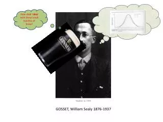
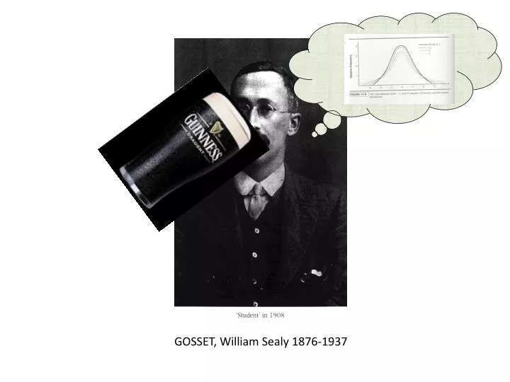
GOSSET, William Sealy 1876-1937. The t-distribution is a family of distributions varying by degrees of freedom ( d.f. , where d.f. = n -1). At d.f. = , but at smaller than that, the tails are fatter. X - . X - . _. _. z = . t = . -. -. X. s X. s. -. s X = . N.

E N D
The t-distribution is a family of distributions varying by degrees of freedom (d.f., where d.f.=n-1). At d.f. =, but at smaller than that, the tails are fatter.
X - X - _ _ z = t = - - X sX s - sX = N
The t-distribution is a family of distributions varying by degrees of freedom (d.f., where d.f.=n-1). At d.f. =, but at smaller than that, the tails are fatter.
Degrees of Freedom df = N - 1
Problem Sample: Mean = 54.2 SD = 2.4 N = 16 Do you think that this sample could have been drawn from a population with = 50?
X - t = - sX Problem Sample: Mean = 54.2 SD = 2.4 N = 16 Do you think that this sample could have been drawn from a population with = 50? _
The mean for the sample of 54.2 (sd = 2.4) was significantly different from a hypothesized population mean of 50, t(15) = 7.0, p < .001.
The mean for the sample of 54.2 (sd = 2.4) was significantlyreliably different from a hypothesized population mean of 50, t(15) = 7.0, p < .001.
SampleC SampleD rXY Population rXY SampleB XY rXY SampleE SampleA _ rXY rXY
r N - 2 t = 1 - r2 The t distribution, at N-2 degrees of freedom, can be used to test the probability that the statistic r was drawn from a population with = 0. Table C. H0 : XY = 0 H1 : XY 0 where