Download
1 / 33
330 likes | 503 Vues
Chapter 4 Digital Transmission. Summary. Topics discussed in previous class. Line Coding Line Coding Schemes Block Coding Scrambling Signal Element versus data element Multilevel : 2b1Q. 4-2 ANALOG-TO-DIGITAL CONVERSION.

E N D
Chapter 4 Digital Transmission
Summary Topics discussed in previous class Line Coding Line Coding Schemes Block Coding Scrambling Signal Element versus data element Multilevel : 2b1Q
4-2 ANALOG-TO-DIGITAL CONVERSION We have seen in Chapter 3 that a digital signal is superior to an analog signal. The tendency today is to change an analog signal to digital data. In this section we describe two techniques, pulse code modulation and delta modulation. Topics discussed in this section: Pulse Code Modulation (PCM)Delta Modulation (DM)
Note According to the Nyquist theorem, the sampling rate must be at least 2 times the highest frequency contained in the signal.
Figure 4.23 Nyquist sampling rate for low-pass and bandpass signals
Example 4.6 For an intuitive example of the Nyquist theorem, let us sample a simple sine wave at three sampling rates: fs = 4f (2 times the Nyquist rate), fs = 2f (Nyquist rate), and fs = f (one-half the Nyquist rate). Figure 4.24 shows the sampling and the subsequent recovery of the signal. It can be seen that sampling at the Nyquist rate can create a good approximation of the original sine wave (part a). Oversampling in part b can also create the same approximation, but it is redundant and unnecessary. Sampling below the Nyquist rate (part c) does not produce a signal that looks like the original sine wave.
Figure 4.24 Recovery of a sampled sine wave for different sampling rates
Example 4.7 Consider the revolution of a hand of a clock. The second hand of a clock has a period of 60 s. According to the Nyquist theorem, we need to sample the hand every 30 s (Ts = T or fs = 2f ). In Figure 4.25a, the sample points, in order, are 12, 6, 12, 6, 12, and 6. The receiver of the samples cannot tell if the clock is moving forward or backward. In part b, we sample at double the Nyquist rate (every 15 s). The sample points are 12, 3, 6, 9, and 12. The clock is moving forward. In part c, we sample below the Nyquist rate (Ts = T or fs = f ). The sample points are 12, 9, 6, 3, and 12. Although the clock is moving forward, the receiver thinks that the clock is moving backward.
Example 4.8 An example related to Example 4.7 is the seemingly backward rotation of the wheels of a forward-moving car in a movie. This can be explained by under-sampling. A movie is filmed at 24 frames per second. If a wheel is rotating more than 12 times per second, the under-sampling creates the impression of a backward rotation.
Example 4.9 Telephone companies digitize voice by assuming a maximum frequency of 4000 Hz. The sampling rate therefore is 8000 samples per second.
Example 4.10 A complex low-pass signal has a bandwidth of 200 kHz. What is the minimum sampling rate for this signal? Solution The bandwidth of a low-pass signal is between 0 and f, where f is the maximum frequency in the signal. Therefore, we can sample this signal at 2 times the highest frequency (200 kHz). The sampling rate is therefore 400,000 samples per second.
Example 4.11 A complex bandpass signal has a bandwidth of 200 kHz. What is the minimum sampling rate for this signal? Solution We cannot find the minimum sampling rate in this case because we do not know where the bandwidth starts or ends. We do not know the maximum frequency in the signal.
Example 4.12 What is the SNRdB in the example of Figure 4.26? Solution We can use the formula to find the quantization. We have eight levels and 3 bits per sample, so SNRdB = 6.02(3) + 1.76 = 19.82 dB Increasing the number of levels increases the SNR.
Example 4.13 A telephone subscriber line must have an SNRdB above 40. What is the minimum number of bits per sample? Solution We can calculate the number of bits as Telephone companies usually assign 7 or 8 bits per sample.
Example 4.14 We want to digitize the human voice. What is the bit rate, assuming 8 bits per sample? Solution The human voice normally contains frequencies from 0 to 4000 Hz. So the sampling rate and bit rate are calculated as follows:
Example 4.15 We have a low-pass analog signal of 4 kHz. If we send the analog signal, we need a channel with a minimum bandwidth of 4 kHz. If we digitize the signal and send 8 bits per sample, we need a channel with a minimum bandwidth of 8 × 4 kHz = 32 kHz.
4-3 TRANSMISSION MODES The transmission of binary data across a link can be accomplished in either parallel or serial mode. In parallel mode, multiple bits are sent with each clock tick. In serial mode, 1 bit is sent with each clock tick. While there is only one way to send parallel data, there are three subclasses of serial transmission: asynchronous, synchronous, and isochronous. Topics discussed in this section: Parallel TransmissionSerial Transmission
Note In asynchronous transmission, we send 1 start bit (0) at the beginning and 1 or more stop bits (1s) at the end of each byte. There may be a gap between each byte.
Note Asynchronous here means “asynchronous at the byte level,” but the bits are still synchronized; their durations are the same.
Note In synchronous transmission, we send bits one after another without start or stop bits or gaps. It is the responsibility of the receiver to group the bits.