Download
1 / 72
820 likes | 1.56k Vues
Multiple Regression – Basic Relationships. Purpose of multiple regression Different types of multiple regression Standard multiple regression Hierarchical multiple regression Stepwise multiple regression Steps in solving regression problems. Purpose of multiple regression.

E N D
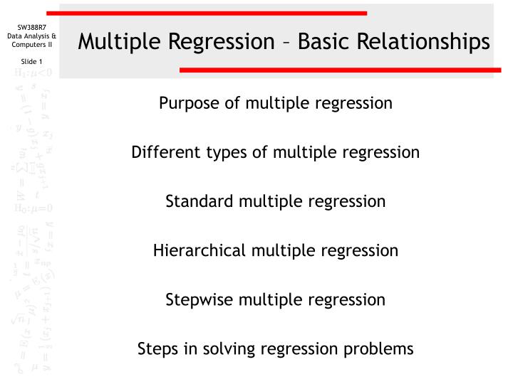
Multiple Regression – Basic Relationships Purpose of multiple regression Different types of multiple regression Standard multiple regression Hierarchical multiple regression Stepwise multiple regression Steps in solving regression problems
Purpose of multiple regression • The purpose of multiple regression is to analyze the relationship between metric or dichotomous independent variables and a metric dependent variable. • If there is a relationship, using the information in the independent variables will improve our accuracy in predicting values for the dependent variable.
Types of multiple regression • There are three types of multiple regression, each of which is designed to answer a different question: • Standard multiple regression is used to evaluate the relationships between a set of independent variables and a dependent variable. • Hierarchical, or sequential, regression is used to examine the relationships between a set of independent variables and a dependent variable, after controlling for the effects of some other independent variables on the dependent variable. • Stepwise, or statistical, regression is used to identify the subset of independent variables that has the strongest relationship to a dependent variable.
Standard multiple regression • In standard multiple regression, all of the independent variables are entered into the regression equation at the same time • Multiple R and R² measure the strength of the relationship between the set of independent variables and the dependent variable. An F test is used to determine if the relationship can be generalized to the population represented by the sample. • A t-test is used to evaluate the individual relationship between each independent variable and the dependent variable.
Hierarchical multiple regression • In hierarchical multiple regression, the independent variables are entered in two stages. • In the first stage, the independent variables that we want to control for are entered into the regression. In the second stage, the independent variables whose relationship we want to examine after the controls are entered. • A statistical test of the change in R² from the first stage is used to evaluate the importance of the variables entered in the second stage.
Stepwise multiple regression • Stepwise regression is designed to find the most parsimonious set of predictors that are most effective in predicting the dependent variable. • Variables are added to the regression equation one at a time, using the statistical criterion of maximizing the R² of the included variables. • When none of the possible addition can make a statistically significant improvement in R², the analysis stops.
Problem 1 - standard multiple regression In the dataset GSS2000.sav, is the following statement true, false, or an incorrect application of a statistic? Assume that there is no problem with missing data, violation of assumptions, or outliers, and that the split sample validation will confirm the generalizability of the results. Use a level of significance of 0.05. The variables "strength of affiliation" [reliten] and "frequency of prayer" [pray] have a strong relationship to the variable "frequency of attendance at religious services" [attend]. Survey respondents who were less strongly affiliated with their religion attended religious services less often. Survey respondents who prayed less often attended religious services less often. 1. True 2. True with caution 3. False 4. Inappropriate application of a statistic
Dissecting problem 1 - 1 When a problem states that there is a relationship between some independent variables and a dependent variable, we do standard multiple regression. 1. In the dataset GSS2000.sav, is the following statement true, false, or an incorrect application of a statistic? Assume that there is no problem with missing data, violation of assumptions, or outliers, and that the split sample validation will confirm the generalizability of the results. Use a level of significance of 0.05. The variables "strength of affiliation" [reliten] and "frequency of prayer" [pray] have a strong relationship to the variable "frequency of attendance at religious services" [attend]. Survey respondents who were less strongly affiliated with their religion attended religious services less often. Survey respondents who prayed less often attended religious services less often. 1. True 2. True with caution 3. False 4. Inappropriate application of a statistic The variables listed first in the problem statement are the independent variables (ivs): "strength of affiliation" [reliten] and "frequency of prayer" [pray] The variable that is related to is the dependent variable (dv): "frequency of attendance at religious services" [attend].
Dissecting problem 1 - 2 • In order for a problem to be true, we will have find: • a statistically significant relationship between the ivs and the dv • a relationship of the correct strength 1. In the dataset GSS2000.sav, is the following statement true, false, or an incorrect application of a statistic? Assume that there is no problem with missing data, violation of assumptions, or outliers, and that the split sample validation will confirm the generalizability of the results. Use a level of significance of 0.05. The variables "strength of affiliation" [reliten] and "frequency of prayer" [pray] have a strong relationship to the variable "frequency of attendance at religious services" [attend]. Survey respondents who were less strongly affiliated with their religion attended religious services less often. Survey respondents who prayed less often attended religious services less often. 1. True 2. True with caution 3. False 4. Inappropriate application of a statistic The relationship of each of the independent variables to the dependent variable must be statistically significant and interpreted correctly.
Request a standard multiple regression To compute a multiple regression in SPSS, select the Regression | Linear command from the Analyze menu.
Specify the variables and selection method First, move the dependent variable attend to the Dependent text box. Second, move the independent variables reliten and pray to the Independent(s) list box. Third, select the method for entering the variables into the analysis from the drop down Method menu. In this example, we accept the default of Enter for direct entry of all variables, which produces a standard multiple regression. Fourth, click on the Statistics… button to specify the statistics options that we want.
Specify the statistics output options First, mark the checkboxes for Estimates on the Regression Coefficients panel. Third, click on the Continue button to close the dialog box. Second, mark the checkboxes for Model Fit and Descriptives.
Request the regression output Click on the OK button to request the regression output.
LEVEL OF MEASUREMENT Multiple regression requires that the dependent variable be metric and the independent variables be metric or dichotomous. "Frequency of attendance at religious services" [attend] is an ordinal level variable, which satisfies the level of measurement requirement if we follow the convention of treating ordinal level variables as metric variables. Since some data analysts do not agree with this convention, a note of caution should be included in our interpretation. "Strength of affiliation" [reliten] and "frequency of prayer" [pray] are ordinal level variables. If we follow the convention of treating ordinal level variables as metric variables, the level of measurement requirement for multiple regression analysis is satisfied. Since some data analysts do not agree with this convention, a note of caution should be included in our interpretation.
SAMPLE SIZE The minimum ratio of valid cases to independent variables for multiple regression is 5 to 1. With 113 valid cases and 2 independent variables, the ratio for this analysis is 56.5 to 1, which satisfies the minimum requirement. In addition, the ratio of 56.5 to 1 satisfies the preferred ratio of 15 to 1.
OVERALL RELATIONSHIP BETWEEN INDEPENDENT AND DEPENDENT VARIABLES - 1 The probability of the F statistic (49.824) for the overall regression relationship is <0.001, less than or equal to the level of significance of 0.05. We reject the null hypothesis that there is no relationship between the set of independent variables and the dependent variable (R² = 0). We support the research hypothesis that there is a statistically significant relationship between the set of independent variables and the dependent variable.
OVERALL RELATIONSHIP BETWEEN INDEPENDENT AND DEPENDENT VARIABLES - 2 The Multiple R for the relationship between the set of independent variables and the dependent variable is 0.689, which would be characterized as strong using the rule of thumb than a correlation less than or equal to 0.20 is characterized as very weak; greater than 0.20 and less than or equal to 0.40 is weak; greater than 0.40 and less than or equal to 0.60 is moderate; greater than 0.60 and less than or equal to 0.80 is strong; and greater than 0.80 is very strong.
RELATIONSHIP OF INDIVIDUAL INDEPENDENT VARIABLES TO DEPENDENT VARIABLE - 1 For the independent variable strength of affiliation, the probability of the t statistic (-5.857) for the b coefficient is <0.001 which is less than or equal to the level of significance of 0.05. We reject the null hypothesis that the slope associated with strength of affiliation is equal to zero (b = 0) and conclude that there is a statistically significant relationship between strength of affiliation and frequency of attendance at religious services.
RELATIONSHIP OF INDIVIDUAL INDEPENDENT VARIABLES TO DEPENDENT VARIABLE - 2 The b coefficient associated with strength of affiliation (-1.138) is negative, indicating an inverse relationship in which higher numeric values for strength of affiliation are associated with lower numeric values for frequency of attendance at religious services. Since both variables are ordinal level, we will have to look at the coding for each before we can make a correct interpretation. For ordinal level variables the numeric codes can be associated with labels in ascending or descending order.
RELATIONSHIP OF INDIVIDUAL INDEPENDENT VARIABLES TO DEPENDENT VARIABLE - 3 The independent variable strength of affiliation is an ordinal variable that is coded so that higher numeric values are associated with survey respondents who were less strongly affiliated with their religion.
RELATIONSHIP OF INDIVIDUAL INDEPENDENT VARIABLES TO DEPENDENT VARIABLE - 4 The dependent variable frequency of attendance at religious services is also an ordinal variable. It is coded so that lower numeric values are associated with survey respondents who attended religious services less often. Therefore, the negative value of b implies that survey respondents who were less strongly affiliated with their religion attended religious services less often.
RELATIONSHIP OF INDIVIDUAL INDEPENDENT VARIABLES TO DEPENDENT VARIABLE - 5 For the independent variable frequency of prayer, the probability of the t statistic (-4.145) for the b coefficient is <0.001 which is less than or equal to the level of significance of 0.05. We reject the null hypothesis that the slope associated with frequency of prayer is equal to zero (b = 0) and conclude that there is a statistically significant relationship between frequency of prayer and frequency of attendance at religious services.
RELATIONSHIP OF INDIVIDUAL INDEPENDENT VARIABLES TO DEPENDENT VARIABLE - 6 The b coefficient associated with how often does r pray (-0.554) is negative, indicating an inverse relationship in which higher numeric values for how often does r pray are associated with lower numeric values for frequency of attendance at religious services. Since both variables are ordinal level, we will have to look at the coding for each before we can make a correct interpretation. For ordinal level variables the numeric codes can be associated with labels in ascending or descending order.
RELATIONSHIP OF INDIVIDUAL INDEPENDENT VARIABLES TO DEPENDENT VARIABLE - 7 The independent variable frequency of prayer is an ordinal variable that is coded so that higher numeric values are associated with survey respondents who prayed less often.
RELATIONSHIP OF INDIVIDUAL INDEPENDENT VARIABLES TO DEPENDENT VARIABLE - 8 The dependent variable frequency of attendance at religious services is also an ordinal variable. It is coded so that lower numeric values are associated with survey respondents who attended religious services less often. Therefore, the negative value of b implies that survey respondents who prayed less often attended religious services less often.
Answer to problem 1 • The independent and dependent variables were metric (ordinal). • The ratio of cases to independent variables was 56.5 to 1. • The overall relationship was statistically significant and its strength was characterized correctly. • The b coefficient for all variables was statistically significant and the direction of the relationships were characterized correctly. • The answer to the question is true with caution. The caution is added because of the ordinal variables.
Problem 2 – hierarchical regression In the dataset GSS2000.sav, is the following statement true, false, or an incorrect application of a statistic? Assume that there is no problem with missing data, violation of assumptions, or outliers, and that the split sample validation will confirm the generalizability of the results. Use a level of significance of 0.05. After controlling for the effects of the variables "age" [age] and "sex" [sex], the addition of the variables "happiness of marriage" [hapmar], "condition of health" [health], and "attitude toward life" [life] reduces the error in predicting "general happiness" [happy] by 36.1%. After controlling for age and sex, the variables happiness of marriage, condition of health, and attitude toward life each make an individual contribution to reducing the error in predicting general happiness. Survey respondents who were less happy with their marriages were less happy overall. Survey respondents who said they were not as healthy were less happy overall. Survey respondents who felt life was less exciting were less happy overall. 1. True 2. True with caution 3. False 4. Inappropriate application of a statistic
Dissecting problem 2 - 1 The variables listed first in the problem statement are the independent variables (ivs) whose effect we want to control before we test for the relationship: "age"[age] and "sex" [sex], 14. In the dataset GSS2000.sav, is the following statement true, false, or an incorrect application of a statistic? Assume that there is no problem with missing data, violation of assumptions, or outliers, and that the split sample validation will confirm the generalizability of the results. Use a level of significance of 0.05. After controlling for the effects of the variables "age" [age] and "sex" [sex], the addition of the variables "happiness of marriage" [hapmar], "condition of health" [health], and "attitude toward life" [life] reduces the error in predicting "general happiness" [happy] by 36.1%. After controlling for age and sex, the variables happiness of marriage, condition of health, and attitude toward life each make an individual contribution to reducing the error in predicting general happiness. Survey respondents who were less happy with their marriages were less happy overall. Survey respondents who said they were not as healthy were less happy overall. Survey respondents who felt life was less exciting were less happy overall. 1. True 2. True with caution 3. False 4. Inappropriate application of a statistic The variables that we add in after the control variables are the independent variables that we think will have a statistical relationship to the dependent variable: "happiness of marriage" [hapmar], "condition of health" [health], and "attitude toward life" [life] The variable that to be predicted or related to is the dependent variable (dv): "general happiness" [happy]
Dissecting problem 2 - 2 In order for a problem to be true, the relationship between the added variables and the dependent variable must be statistically significant, and the strength of the relationship after including the control variables must be correctly stated. 14. In the dataset GSS2000.sav, is the following statement true, false, or an incorrect application of a statistic? Assume that there is no problem with missing data, violation of assumptions, or outliers, and that the split sample validation will confirm the generalizability of the results. Use a level of significance of 0.05. After controlling for the effects of the variables "age" [age] and "sex" [sex], the addition of the variables "happiness of marriage" [hapmar], "condition of health" [health], and "attitude toward life" [life] reduces the error in predicting "general happiness" [happy] by 36.1%. After controlling for age and sex, the variables happiness of marriage, condition of health, and attitude toward life each make an individual contribution to reducing the error in predicting general happiness. Survey respondents who were less happy with their marriages were less happy overall. Survey respondents who said they were not as healthy were less happy overall. Survey respondents who felt life was less exciting were less happy overall. 1. True 2. True with caution 3. False 4. Inappropriate application of a statistic The relationship between each of the independent variables entered after the control variables and the dependent variable must be statistically significant and interpreted correctly. We are generally not interested in whether or not the control variables have a statistically significant relationship to the dependent variables.
Request a hierarchical multiple regression To compute a multiple regression in SPSS, select the Regression | Linear command from the Analyze menu.
Specify independent variables to control for First, move the dependent variable happy to the Dependent text box. Second, move the independent variables to control for age and sex to the Independent(s) list box. Fourth, click on the Next button to tell SPSS to add another block of variables to the regression analysis. Third, select the method for entering the variables into the analysis from the drop down Method menu. In this example, we accept the default of Enter for direct entry of all variables in the first block which will force the controls into the regression.
Add the other independent variables SPSS identifies that we will now be adding variables to a second block. First, move the other independent variables hapmar, health and life to the Independent(s) list box for block 2. Second, click on the Statistics… button to specify the statistics options that we want.
Specify the statistics output options First, mark the checkboxes for Estimates on the Regression Coefficients panel. Third, click on the Continue button to close the dialog box. Second, mark the checkboxes for Model Fit, Descriptives, and R squared change. The R squared change statistic will tell us whether or not the variables added after the controls have a relationship to the dependent variable.
Request the regression output Click on the OK button to request the regression output.
LEVEL OF MEASUREMENT Multiple regression requires that the dependent variable be metric and the independent variables be metric or dichotomous. "General happiness" [happy] is an ordinal level variable, which satisfies the level of measurement requirement if we follow the convention of treating ordinal level variables as metric variables. Since some data analysts do not agree with this convention, a note of caution should be included in our interpretation. "Age" [age] is an interval level variable, which satisfies the level of measurement requirements for multiple regression analysis. "Happiness of marriage" [hapmar], "condition of health" [health], and "attitude toward life" [life] are ordinal level variables. If we follow the convention of treating ordinal level variables as metric variables, the level of measurement requirement for multiple regression analysis is satisfied. Since some data analysts do not agree with this convention, a note of caution should be included in our interpretation. "Sex" [sex] is a dichotomous or dummy-coded nominal variable which may be included in multiple regression analysis.
SAMPLE SIZE The minimum ratio of valid cases to independent variables for multiple regression is 5 to 1. With 90 valid cases and 5 independent variables, the ratio for this analysis is 18.0 to 1, which satisfies the minimum requirement. In addition, the ratio of 18.0 to 1 satisfies the preferred ratio of 15 to 1.
OVERALL RELATIONSHIP BETWEEN INDEPENDENT AND DEPENDENT VARIABLES The probability of the F statistic (9.493) for the overall regression relationship for all indpendent variables is <0.001, less than or equal to the level of significance of 0.05. We reject the null hypothesis that there is no relationship between the set of all independent variables and the dependent variable (R² = 0). We support the research hypothesis that there is a statistically significant relationship between the set of all independent variables and the dependent variable.
REDUCTION IN ERROR IN PREDICTING DEPENDENT VARIABLE - 1 The R Square Change statistic for the increase in R² associated with the added variables (happiness of marriage, condition of health, and attitude toward life) is 0.361. Using a proportional reduction in error interpretation for R², information provided by the added variables reduces our error in predicting general happiness by 36.1%.
REDUCTION IN ERROR IN PREDICTING DEPENDENT VARIABLE - 2 The probability of the F statistic (15.814) for the change in R² associated with the addition of the predictor variables to the regression analysis containing the control variables is <0.001, less than or equal to the level of significance of 0.05. We reject the null hypothesis that there is no improvement in the relationship between the set of independent variables and the dependent variable when the predictors are added (R² Change = 0). We support the research hypothesis that there is a statistically significant improvement in the relationship between the set of independent variables and the dependent variable.
RELATIONSHIP OF ADDED INDEPENDENT VARIABLES TO DEPENDENT VARIABLE - 1 If there is a relationship between each added individual independent variable and the dependent variable, the probability of the statistical test of the b coefficient (slope of the regression line) will be less than or equal to the level of significance. The null hypothesis for this test states that b is equal to zero, indicating a flat regression line and no relationship. If we reject the null hypothesis and find that there is a relationship between the variables, the sign of the b coefficient indicates the direction of the relationship for the data values. If b is greater than or equal to zero, the relationship is positive or direct. If b is less than zero, the relationship is negative or inverse. If the variable is dichotomous or ordinal, the direction of the coding must be taken into account to make a correct interpretation.
RELATIONSHIP OF ADDED INDEPENDENT VARIABLES TO DEPENDENT VARIABLE - 2 For the independent variable happiness of marriage, the probability of the t statistic (5.741) for the b coefficient is <0.001 which is less than or equal to the level of significance of 0.05. We reject the null hypothesis that the slope associated with happiness of marriage is equal to zero (b = 0) and conclude that there is a statistically significant relationship between happiness of marriage and general happiness.
RELATIONSHIP OF ADDED INDEPENDENT VARIABLES TO DEPENDENT VARIABLE - 3 The b coefficient associated with happiness of marriage (0.599) is positive, indicating a direct relationship in which higher numeric values for happiness of marriage are associated with higher numeric values for general happiness.
RELATIONSHIP OF ADDED INDEPENDENT VARIABLES TO DEPENDENT VARIABLE - 4 The independent variable happiness of marriage is an ordinal variable that is coded so that higher numeric values are associated with survey respondents who were less happy with their marriages.
RELATIONSHIP OF ADDED INDEPENDENT VARIABLES TO DEPENDENT VARIABLE - 5 The dependent variable general happiness is also an ordinal variable. It is coded so that higher numeric values are associated with survey respondents who were less happy overall. Therefore, the positive value of b implies that survey respondents who were less happy with their marriages were less happy overall.
RELATIONSHIP OF ADDED INDEPENDENT VARIABLES TO DEPENDENT VARIABLE - 6 For the independent variable condition of health, the probability of the t statistic (1.408) for the b coefficient is 0.163 which is greater than the level of significance of 0.05. We fail to reject the null hypothesis that the slope associated with condition of health is equal to zero (b = 0) and conclude that there is not a statistically significant relationship between condition of health and general happiness. The statement in the problem that "survey respondents who said they were not as healthy were less happy overall" is incorrect.
Answer to problem 2 • The independent and dependent variables were metric or dichotomous. Some are ordinal. • The ratio of cases to independent variables was 18.0 to 1. • The overall relationship was statistically significant and its strength was characterized correctly. • The change in R2 associated with adding the second block of variables was statistically significant and correctly interpreted. • The b coefficient for happiness of marriage was statistically significant and correctly interpreted. The b coefficient for condition of health was not statistically significant. We cannot conclude that there was a relationship between condition of health and general happiness. • The answer to the question is false.
Problem 3 – Stepwise Regression 26. In the dataset GSS2000.sav, is the following statement true, false, or an incorrect application of a statistic? Assume that there is no problem with missing data, violation of assumptions, or outliers, and that the split sample validation will confirm the generalizability of the results. Use a level of significance of 0.05. From the list of variables "number of hours worked in the past week" [hrs1], "occupational prestige score" [prestg80], "highest year of school completed" [educ], and "highest academic degree" [degree], the best predictors of "total family income" [income98] are "highest academic degree" [degree] and "occupational prestige score" [prestg80]. Highest academic degree and occupational prestige score have a moderate relationship to total family income. The most important predictor of total family income is occupational prestige score. The second most important predictor of total family income is highest academic degree. Survey respondents who had higher academic degrees had higher total family incomes. Survey respondents who had more prestigious occupations had higher total family incomes. 1. True 2. True with caution 3. False 4. Inappropriate application of a statistic
Dissecting problem 3 - 1 The variables listed first in the problem statement are the independent variables from which the computer will select the best subset using statistical criteria. The variable that to be predicted or related to is the dependent variable (dv): "total family income" [income98] 26. In the dataset GSS2000.sav, is the following statement true, false, or an incorrect application of a statistic? Assume that there is no problem with missing data, violation of assumptions, or outliers, and that the split sample validation will confirm the generalizability of the results. Use a level of significance of 0.05. From the list of variables "number of hours worked in the past week" [hrs1], "occupational prestige score" [prestg80], "highest year of school completed" [educ], and "highest academic degree" [degree], the best predictors of "total family income" [income98] are "highest academic degree" [degree] and "occupational prestige score" [prestg80]. Highest academic degree and occupational prestige score have a moderate relationship to total family income. The most important predictor of total family income is occupational prestige score. The second most important predictor of total family income is highest academic degree. Survey respondents who had higher academic degrees had higher total family incomes. Survey respondents who had more prestigious occupations had higher total family incomes. 1. True 2. True with caution 3. False 4. Inappropriate application of a statistic The best predictors are the variables that will be meet the statistical criteria for inclusion in the model.
Dissecting problem 3 - 2 • In order for a problem to be true, we will have find: • a statistically significant relationship between the included ivs and the dv • a relationship of the correct strength 26. In the dataset GSS2000.sav, is the following statement true, false, or an incorrect application of a statistic? Assume that there is no problem with missing data, violation of assumptions, or outliers, and that the split sample validation will confirm the generalizability of the results. Use a level of significance of 0.05. From the list of variables "number of hours worked in the past week" [hrs1], "occupational prestige score" [prestg80], "highest year of school completed" [educ], and "highest academic degree" [degree], the best predictors of "total family income" [income98] are "highest academic degree" [degree] and "occupational prestige score" [prestg80]. Highest academic degree and occupational prestige score have a moderate relationship to total family income. The most important predictor of total family income is occupational prestige score. The second most important predictor of total family income is highest academic degree. Survey respondents who had higher academic degrees had higher total family incomes. Survey respondents who had more prestigious occupations had higher total family incomes. 1. True 2. True with caution 3. False 4. Inappropriate application of a statistic The importance of the variables is provided by the stepwise order of entry of the variable into the regression analysis.
Dissecting problem 3 - 3 26. In the dataset GSS2000.sav, is the following statement true, false, or an incorrect application of a statistic? Assume that there is no problem with missing data, violation of assumptions, or outliers, and that the split sample validation will confirm the generalizability of the results. Use a level of significance of 0.05. From the list of variables "number of hours worked in the past week" [hrs1], "occupational prestige score" [prestg80], "highest year of school completed" [educ], and "highest academic degree" [degree], the best predictors of "total family income" [income98] are "highest academic degree" [degree] and "occupational prestige score" [prestg80]. Highest academic degree and occupational prestige score have a moderate relationship to total family income. The most important predictor of total family income is occupational prestige score. The second most important predictor of total family income is highest academic degree. Survey respondents who had higher academic degrees had higher total family incomes. Survey respondents who had more prestigious occupations had higher total family incomes. 1. True 2. True with caution 3. False 4. Inappropriate application of a statistic The relationship between each of the independent variables entered after the control variables and the dependent variable must be statistically significant and interpreted correctly. Since statistical significance of a variable's contribution toward explaining the variance in the dependent variable is almost always used as the criteria for inclusion, the statistical significance of the relationships is usually assured.