Solving Multivariate Polynomial Systems with Hyperplane Arithmetic
440 likes | 506 Vues
Explore solving polynomial systems using hyperplane arithmetic and linear programming for applications like Apollonius Problem, Voronoi diagrams, kinematics, and more. Learn about interval arithmetic, multivariate bisection algorithm, Bezier/B-spline solvers, and research questions on domain reduction and tensor representation.

Solving Multivariate Polynomial Systems with Hyperplane Arithmetic
E N D
Presentation Transcript
Solving Multivariate Polynomial Systemsusing Hyperplane Arithmetic and Linear Programming IddoHanniel
The Problem Consider the following set ofnpolynomial equations: inRn. We seek the simultaneous solution, , such that for alli =1,…,n.
Apollonius Problem Applications Voronoi diagram of circles Artillery sound range locator 4
Example Voronoi Diagram Vertices p 2 distance constraint + 3 tangency constraint = 5 equations in 5 unknowns (can we do in less?) 5
Previous Work on Multivariate Polynomial Solvers Algebraic Solvers: Grobner bases [Cox et al., 1992]. Multivariate Sturm sequences [Milne, 1992]. Homotopy methods [Wampler 05]. Subdivision Solvers: Interval arithmetic solvers [Merlet 2000] Subdivision solvers based on the Bernstein/Bezier/B-spline properties [Sherbrooke and Patrikalakis, 1993], [Elber and Kim, 2001]. 7
Interval Arithmetic For two intervals [a, b] and [c, d] that are subsets of (-∞,+ ∞): [a, b] + [c, d] = [a + c, b + d] [a, b] − [c, d] = [a − d, b − c] [a, b] × [c, d] = [min (a × c, a × d, b × c, b × d), max (a × c, a × d, b × c, b × d)] [a, b] ÷ [c, d] = [min (a ÷ c, a ÷ d, b ÷ c, b ÷ d), max (a ÷ c, a ÷ d, b ÷ c, b ÷ d)] when 0 is not in [c, d]. 8
Interval of Powers Odd n: Even n: 9
Interval Based Multivariate Bisection Algorithm root_isolation_in_box(Multivariate F(x1,..,xn), Box B[a1,b1]×.. ×[an,bn], Output {Boxes}) If (max(bi-ai) < ε) append B to output boxes and return. Evaluate [Fmin,Fmax] = F([a1,b1], ..,[an,bn]). If [Fmin,Fmax] does not contain 0, return. Split B into two sub-boxes, B1,B2 at 0.5(bm+am), where m = {i: (bi-ai) is maximal}. root_isolation_in_box(F,B1,{Boxes}) root_isolation_in_box(F,B2,{Boxes}) 10
The Basic Bezier/B-Spline Solver A subdivision step in a multidimensional space, using B-spline/Bezier subdivision. A multivariate Newton-Raphson (NR)numeric step. [Elber and Kim, 2001] 12
Subdivision Illustration – Univariate Case Subdivision. CH containment. 13
Basic Bezier Based Multivariate Subdivision Algorithm root_isolation_in_box(Multivariate F(x1,..,xn), Box B[a1,b1]×.. ×[an,bn], Output {Boxes}) • If (max(bi-ai) < ε) append B to output boxes and return. • If CH does not contain 0, return. • Split B into two sub-boxes, B1,B2 at 0.5(bm+am), where m = {i: (bi-ai) is maximal}. • root_isolation_in_box(F,B1,{Boxes}) • root_isolation_in_box(F,B2,{Boxes}) 15
Research Questions When do we stop the subdivision? Single solution test [Hanniel & Elber 07, Wei et al. 11]. • Can we handle univariate solutions? [Barton, Hanniel & Elber 11] • What about bivariate solutions? [Mizrahi & Elber 15] • Can preconditioning improve the algorithm? [Mourrain & Pavone 09] • Can we reduce the domain more efficiently? • Projected Polyhedron [Sherbrooke & Patrikalakis 93]. • Projected curves [Mourrain & Pavone 09]. • Linear Programming on Bernstein Polyhedra [Funfzig et al. 09] 16
Domain Reduction using Bounding Hyperplanes The basic idea: Bound the function Fi=0 by a pair of parallel hyper-planes in Rd. The root can only be at the intersection of the bounding hyperplanes. F1 F2 17
Linear Programming Under a set of linear constraints (inequalities) of type: Maximize the linear objective function of type: 18
Linear Programming Example Constraints: • Maximize f(x1,x2)=x2 • Maximize f(x1,x2)=x1 19
Bounding Hyperplane Construction • Promote Fi from a scalar function to a hyper-surface in Rn+1, . • Evaluate the gradient (i.e., the normal) at the sub-domain mid-point and project all control points of the hyper-surface onto it. • The two hyper-planes orthogonal to the gradient and passing through the extreme projection points, bound Fi. 20
Bounding Hyperplane Construction Illustration (d=1) [ ] xn+1 = 0 21
Domain Reduction Procedure using LP Bound Fi from above and below by two hyperplanes: HPmin ≤Fi ≤HPmax . Perform 2n LP queries (for objective functions min/maxxi ). Reduce the domain to box with min/maxxi. 22
Why is Tensor Representation a Problem? [Bamberger and Shoham, 2007] 23
Why is Tensor Representation a Problem? Grows exponentially with number of variables n (O(l+1)n). Dense representation: Even for sparse systems, all coefficients are required for Bezier properties (e.g., CH). Standard power form requires only O(nl) and in many cases less (e.g., linear, constant). 24
Research Question Can we use a sparse representation and still benefit the features of Bezier representation? Previous work: • Elber & Grandine 09: Expression Trees • Funfzig et al. 09: Bernstein polyhedra and LP 25
From Interval Arithmetic to Hyperplane Arithmetic Interval arithmetic: • Generalization to bounding functions:
Hyperplane Arithmetic Example • Bounding sum: • Bounding first monom: • Bounding second monom:
Hyperplane Arithmetic Example x1 - 0.25 ≤ x12≤x1 x2 - 0.25 ≤ x22≤ x2 x1 + x2 – 1.5 ≤x12 + x22 - 1≤x1+x2– 1
LP Algorithm using Hyperplane Arithmetic Bound Fi polynomials by two parallel hyperplanes, using hyperplane arithmetic of bounds on its monomial terms. Perform 2n LP computations to compute new [ximin,ximax] values for each xi. Continue recursively on the new reduced domain.
Experimental Results Tested Algorithms: • IRIT Naïve - basic with mid parameter subdivision – no reduction. • IRIT PP - variant of [Sherbrooke & Patrikalakis 93]. • Bernst LP - variant of [Funfzig et al. 09]. • Naïve LP - our algorithm with dense Bezier representation. • HPA LP - our algorithm with hyper-plane arithmetic. Test cases: • Easily scalable by number of variables • Easily computable roots. 30
Experimental Results – Hyper-cylinders What does it look like? How many roots are there? 31
Results Hyper-cylinders (I) ms 32 n
Results Hyper-cylinders (II) ms 33 n
Results – Degree 3 (I) ms 35 n
Results – Degree 3 (Opt vs. No Opt) ms n Tighter (optimized) bounding hyperplanes specialized for x3. 36
Broyden Tridiagonal System • Classic function in optimization community (where not all root are necessarily required). • Easily scaled by number of variables. • Two roots in [-2,2]n . 37
Broyden Results (I) ms 38 n
Broyden Results (II) ms 39 n
A Dense System • Taken from [Tsidon, Hanniel & Kesslassi 2012]. • Dense system easily scaled by number of variables. • One root in (0,1]n . 40
Dense System (cont.) Solution formula: What does the geometry of these surfaces look like?
Results – Dense System ms 42 n