Download
1 / 37
400 likes | 992 Vues
Confounding. Confounding is an apparent association between disease and exposure caused by a third factor not taken into consideration A confounder is a variable that is associated with the exposure and, independent of that exposure, is a risk factor for the disease. Examples.

E N D
Confounding • Confounding is an apparent association between disease and exposure caused by a third factor not taken into consideration • A confounder is a variable that is associated with the exposure and, independent of that exposure, is a risk factor for the disease
Examples • Study A found an association between cigar smoking and baldness • The study was confounded by age • Study B found a protective effect between animal companions and heart attack • The study may be confounded by the fact that pets require care and pet owners were more active or able to physically care for them • The study may also be confounded by the fact that those who can tolerate pets are more easy-going (Type B personalities) • Study C found improved perinatal outcomes for birthing centers when compared to hospitals • The study may be confounded by highly motivated volunteers who select the birthing center option
Testing for Confounding • Obtain a crude outcome measure (crude death rate, crude birth rate, overall odds ratio or relative risk) • Repeat the outcome measure controlling for the variable (age-adjusted rate, gender- specific odds ratio or relative risk) • Compare the two measures; the estimate of the two measures will be different if the variable is a confounder
Testing for Confounding (cont.) Age Std Pop* Expected ASR/1,000 Cancer Deaths Pop At Risk Young 5 5,000 1.00 60,500 Middle 10 25,000 0.40 140,300,000 56,120 Old 15,000 6.67 25,700,000 171,419 100 Total 115 45,000 XXXX 288,039 226,500,000 * 1980 Population of the U.S., where Young = 0-18, Middle = 19-64, Old = 65+ Crude Rate= Total Deaths / Pop At Risk = 115 / 45,000 = 2.56 / 1,000 AAR = Sum of Expected / Total in Std Pop = 1.27 / 1,000 AGE IS A CONFOUNDER FOR DEATH FROM CANCER
Controls for Confounding • Controls for confounding may be built into the design or analysis stages of a study • Design stage • Randomization (For Experimental Studies) • Restriction (Allow only those into the study who fit into a narrow band of a potentially confounding variable) • Matching (Match cases and controls on the basis of the potential confounding variables – especially age and gender) • Cases and controls can be individually matched for one or more variables, or they can be group matched • Matching is expensive and requires specific analytic techniques • Overmatching or unnecessary matching may mask findings
Controls for Confounding (cont) • Analysis Stage • Stratification • Multivariate Analysis – Multiple Linear Regression, Logistic Regression, Proportional Hazards Model
Testing for Effect Modification (Interaction among variables) • When the incidence rate of disease in the presence of two or more risk factors differs from the incidence rate expected to result from their individual effects • The effect can be greater than would be expected (positive interaction, synergism) or less than would be expected (negative interaction, antagonism)
Effect Modification (Interaction), cont. • To assess interaction: • Is there an association? • If so, is it due to confounding? • If not, are there differences in strata formed on the basis of a third variable? • If so, interaction or effect modification is present • If not, there is no interaction or effect modification
The prevalence of osteoarthritisis 50% among females at age 65. Are Ca supplements beginning at age 50 helpful? Those with treatment had 84% less disease at age 65
Did smoking confound the Ca treatment? Disease No Disease Non-smokers Ca+ 20 320 340 Ca- 80 80 160 RR=0.12 100 400 500 Disease No Disease Ca+ 30 130 160 Smokers Ca- 270 70 340 RR=0.24 300 200 500
Was treatment for smokers modified by alcohol? Disease No Disease Ca+ 25 75 100 Ca- 250 50 300 RR=0.30 275 125 400 Smokers who drink Disease No Disease Ca+ 5 55 60 RR=0.17 Ca- 20 20 40 25 75 100 Smokers who do not drink
Assessing the Relationship Between a Possible Cause and an Outcome OBSERVED ASSOCIATION 2. Could it be due to confounding or effect modification? 1. Could it be due to selection or information bias? NO NO 3.Could it be a result of the role of chance? PROBABLY NOT 4. Could it be causal? Apply guidelines and make judgment
Evaluating an Association • How can we be sure that what we have found is a true association – to build a case for cause? • Epidemiologists go through a 3 step process • Examine the methodology for bias • Examine the analysis for confounding and effect modification • Examine the results for statistical significance
Inferential Statistics • Allow for making predictions, estimations or inferences about what has not been observed based on what has (from a sample) through hypothesis testing
Inferential Statistics • Requires testing a hypothesis • Ho: null hypothesis • No effect or no difference • Ha: research (alternative) hypothesis • There is an effect or difference
Statistical Significance • I believe that Treatment A is better than Treatment B. Why not test my research hypothesis? Why test the null hypothesis? H0 : Treatment A = Treatment B • The research hypothesis requires an infinite number of statistical tests • If we test the null hypothesis, we only have to perform one test, that of no difference
Steps in Hypothesis Testing (cont.) • A statistical association tells you the likelihood the result you obtained happened by chance alone • A strong statistical association does not show cause! • Every time we reject the null hypothesis we risk being wrong • Every time we fail to reject the null hypothesis we risk being wrong
Examples of Hypothesis Testing • We calculated age-adjusted rates for San Francisco and San Jose and compared them • Ho: AAR1 = AAR2 • Ha: There is a statistically significant difference between the age-adjusted rates of San Francisco and San Jose
Hypothesis Testing (cont.) • We calculated odds ratios and relative risks • Ho: OR = 1 (or RR = 1) • Ha: There is a statistically significant difference between cases and controls (or between the exposed and unexposed)
Hypothesis Testing (cont.) • We calculated the SMR for farmers • Ho: SMR = 100% • Ha: There is a statistically significant difference between the cohort and the control population
Steps in Hypothesis Testing • Assume the null hypothesis is true • Collect data and test the difference between the two groups • The probability that you would get these results by chance alone is the p-value • If the p-value is low (chance is an improbable explanation for the result), reject the null hypothesis
Null Hypothesis • H0: Treatment A (single-dose treatment for UTI) = Treatment B (multi-dose treatment for UTI) • Set alpha at .05 (1 in 20 chance of a Type I Error) • You calculate a p-value (the probability that what you found was by chance) of .07 • You fail to reject the null hypothesis • The difference between the groups was not statistically significant • Are the findings clinically important?
Null Hypothesis • There is nothing magical about an alpha of .05 or .01 • There are situations where an alpha of .20 is acceptable • The size of the p-value does not indicate the importance of the results • The p-value tells us the probability that we have made a mistake – that we rejected the null hypothesis and claimed a difference when there was none • Results may be statistically significant but be clinically unimportant • Results that are not statistically significant may still be important
Confidence Interval • Sometimes we are more concerned with estimating the true difference than the probability that we are making the right decision (p-value) • The .95 confidence interval provides the interval in which the true value is likely to be found 95 percent of the time • If the confidence limit contains 0 or 1 (the value of no difference) we cannot reject the null hypothesis • Larger sample sizes yield smaller confidence intervals – more confidence in the results
Are these rates statistically significantly different from each other? The 95% confidence intervals tell you. AAR1 = 346.9 (SE 2.5) (344.4, 349.4) AAR2 = 327.8 (SE 14) (313.8, 341.8)
AAR1 was statistically significantly higher than AAR2What about these? SMR = 112% (99, 125) RR = 3.4 (1.2, 5.6)
Every time we use inferential statistics we risk being wrong
Ways to be wrong • TYPE I ERROR – rejecting the null when the null is true – there is no difference • TYPE II ERROR – failing to reject the null when the null is false – there is a difference
Power of the Test • Beta (the probability of a Type II Error) is important if we don’t want to miss an effect • We can reduce the risk of Type II Error by improving the power of the test • Power: The likelihood you will detect an effect of a particular size based on a particular number of subjects
Power of the Test • Power is influenced by: • The significance level (probability of a Type I Error) you set for the hypothesis test; • The size of the difference you wish to detect • The number of subjects in the study
Subjects in the Study • More subjects allows for determining smaller differences • More subjects yields smaller confidence intervals • More subjects cost more money • More subjects increases the complexity of the project • Do you need more subjects?
Maybe! Balance the Following: • Finding no significant difference in a small study tells us nothing • Finding a significant difference in a small study may not be able to be replicated because of sampling variation • Finding no significant difference in a large study tells us treatments or outcomes are essentially equivalent • Finding a significant difference in a large study reveals a true difference, but the findings may not be clinically important
How Do I Figure Out What to Do? • Go to the literature to estimate the incidence or prevalence of the disease (or rate of recovery) in the control population OR • Estimate the exposure (treatment, screening) in the control population • Determine what difference you wish to detect between the control and study populations • Select an alpha – the risk of finding an effect when there really isn’t one (usually .05 or .01) • Select a power level – the probability of finding an effect when there really is one (usually .80 or .90) • Calculate or use sample size tables to determine how many subjects you will need
Finally, can you get that many subjects with your budget, time, and logistical constraints? If not, the study is probably not worth doing unless you will accept a lower power or a larger alpha
H0 : Treatment A = Treatment B Sample Size for a Clinical Trial (1-tail vs. 2-tail test, by which we wish to test increased or decreased survival with Treatment B) Sample Size Required for Each Group Survival with Treatment A Survival with Treatment B Significance Level Power .05 1-tail 30% 10% increase or decrease .80 280 .05 2-tail 30% 10% increase or decrease .80 356 .05 1-tail 30% 20% increase or decrease .80 73 .05 2-tail 30% 20% increase or decrease .80 92
H0 : Treatment A = Treatment B Sample Size for a Clinical Trial (1-tail test, varying the significance level, power and difference we wish to detect) Sample Size Required for Each Group Significance Level Survival with Treatment A Survival with Treatment B Power 10% difference 280 .05 30% .80 73 20% difference 10% difference 388 .05 30% .90 20% difference 101 10% difference .01 30% .80 455 118 20% difference 10% difference 590 .01 30% .90 20% difference 153