Download
1 / 44
440 likes | 445 Vues
This paper discusses the construction of min-cost binary comparison search trees and presents new results in the field. It explores the history, different types of trees, and dynamic programming algorithms for constructing optimal trees. The main lemma and structural properties of the trees are also covered. The paper concludes with extensions and open problems.

E N D
New Results on Binary Comparison Search Trees • Marek Chrobak, Neal Young • UC Riverside • Mordecai Golin • HKUST • Ian Munro U Waterloo
Early version of paper at arxiv.org Optimal search trees with 2-way comparisonsMarek Chrobak, Mordecai Golin, J. Ian Munro, Neal E. YoungarXiv:1505.00357
Main Result • Constructing Min-Cost Binary Comparison Search Trees • Wasn’t this completely understood 45 years ago??!! • Yes and No …
Outline • History • Binary Search Trees • Hu-Tucker Trees • AKKL Trees • Optimal Binary Comparison Search Trees with Failures • Problem Models • List of New Results • New Results • The Main Lemma • Structural Properties of OBCSTs • Dynamic Programming for OBCSTs • Proof of The Main Lemma (Sketch) • Extensions and Open Problems
Knuth [1971] gave algorithm for constructing Optimal Binary Search Trees Known: n keys K1, K2, …., Kn. Preprocess keys to create binary tree. Tree query compares query value Q to keys. and returns appropriate response from i such that Q = Ki i such that Ki < Q < Ki+1 Q < K1 or Kn < Q Input: probability of successful and unsuccessful searches Knuth’s Optimal BSTs
Knuth [1971] gave algorithm for constructing Optimal Binary Search Trees Input was probability of successful and unsuccessful searches Cost of tree was average path length Dynamic Programming Algorithm Constructed O(n^2) DP table Knuth reduced O(n^3) running time to O(n^2) Technique later generalized as Quadrangle Inequality method by F. Yao Knuth’s Optimal BSTs
Knuth’s Optimal BSTs • Cost = 0.85 • Cost = 1.10 • Cost = 0.80 • Cost = 1.05
Hu-Tucker Binary Comparison Search Trees Knuth constructed optimal binary search trees • Trees structure was binary but nodes used ternary comparisons. Each node needed two binary comparisons to implement the search • In a binary comparison search tree, each internal node performs only one comparison. Searches all terminate at leaves. • First such trees constructed by Hu-Tucker, also in 1971. O(n log n)
Hu-Tucker Binary Comparison Search Trees • Hu Tucker (1971) & Garsia-Wachs (1977) • Assumes all searches are successful; no failures allowed. Input is only β1, β2, …, βn, with no αi s. • Internal nodes are < comparisons.Searches all terminate at leaves • Problem is to find tree with minimum weighted (average) external path length • O(n log n) algorithm
Outline • History • Binary Search Trees • Hu-Tucker Trees • AKKL Trees • Optimal Binary Comparison Search Trees with Failures • Problem Models • List of New Results • New Results • The Main Lemma • Structural Properties of OBCSTs • Dynamic Programming for OBCSTs • Proof of The Main Lemma (Sketch) • Extensions and Open Problems
Adding Equality Comparisons • The Knuth trees use three-way comparisons at each node. • These are implemented in modern machines using two two-way comparisons (one < and one =). • Hu-Tucker trees use only one two-way comparison (a <) at each node. • . . . machines that cannot make three-way comparisons at once. . . will have to make two comparisons. . . it may well be best to have a binary tree whose internal nodes specify either an equality test or a less-than test but not both. • D. E. Knuth. The Art of Computer Programming, Volume 3: Sorting and Searching. • Addison-Wesley, 2nd edition, 1998. [§6.2.2 ex. 33],
Adding Equality Comparisons: AKKL[2001] • Hu-Tucker Tree • AKKL Tree • AKKL trees are min cost trees with more power. instead of being restricted to be <, comparisons can be = OR < • AKKL trees include HT Trees • AKKL trees can be cheaper than HT Trees if some βimuch larger than others • AKKL trees more difficult to construct
Adding Equality Comparisons: AKKL[2001] • Anderson, Kannan, Karloff, Ladner [2002] extended Hu-Tucker by allowing = comparisons. AKKL find min-cost tree when the n-1 internal node comparisons are allowed to be in {=,<}. • Useful when some βi are very large (relatively) • AKKL algorithm runs in O(n4) time. • AKKL note this improves running time of O(n5) claimed by Spuler [1994] in his thesis • Spuler only states O(n5) algorithm but doesn’t prove that it produces optimal tree, so AKKL is really first polynomial time algorithm • Reason problem is difficult is that equality nodes can create holes in ranges. This could dramatically (exponentially?) increase search space, destroying DP approach • AKKL show that if equality comparison exists, then it is always largest probability in range. Allows recovering DP approach with ranges of description size O(n3) (compared to Knuth’s O(n2))
Adding Equality Comparisons: AKKL[2001] • Hu-Tucker Tree • AKKL Tree • Comment 1 : Other problem in AKKL is how to deal with repeated weights • This was hardest part. • Comment 2: Both Hu-Tucker and AKKL only work when failures don’t occur.I.e., only βi are allowed and not αi.
So Far + Obvious Open Problem • Optimal Binary Search Trees • Input: • O(n2) Knuth • Optimal Binary Comparison Search Trees • Input: • C = {<}: O(n logn) Hu-Tucker & Garsia-Wachs • C = {=,<}: O(n4) AKKL • Obvious Questions • Can we build OBCSTs that allow failures? • If yes, for which sets of comparisons? • Answer is yes, (for all sets of comparisons) but first need to define problem models
Outline • History • Binary Search Trees • Hu-Tucker Trees • AKKL Trees • Optimal Binary Comparison Search Trees with Failures • Problem Models • List of New Results • New Results • The Main Lemma • Structural Properties of OBCSTs • Dynamic Programming for OBCSTs • Proof of The Main Lemma (Sketch) • Extensions and Open Problems
BCSTs with Failure Probabilities • Allows Failures (βi and αi). • Call this complete input. HT has restricted input. • Tree for n keys has 2n+1 leaves • Distinguishing between Q==Kiand Ki < Q < Ki+1 always requires querying (Q=Ki)
Using Different Types of Comparisons • Left Tree uses {<,=}. Right Tree uses {<, ≤, =} • Minimum cost BCST is minimum taken over all trees using given set of comparisons C, e.g., C={<,=} or C={<, ≤, =} • C is input to the problem. • Algorithm is different for different Cs.
How Much Information is Needed for Failure? Comparisons • Tree on left shows Explicit Failure • every failure leaf reports unique failure interval, Ki < Q < Ki+1. • Tree on right shows Non-Explicit Failure: • Failure leaves only report failure. Don’t need to specify exact interval. Leaf can be concatenation of successive failure intervals .
New Algorithms: OBCSTs with Failures FFFailueComparisons • DP Algorithms for last 4 cases are very similar • Differ slightly in • Design of Recurrence Relations • {=,<} and {=,<, ≤) yield slightly different recurrences • Initial conditions • Explicit and Non-Explicit Failures force different I.C.s
Outline • History • Binary Search Trees • Hu-Tucker Trees • AKKL Trees • Optimal Binary Comparison Search Trees with Failures • Problem Models • List of New Results • New Results • The Main Lemma • Structural Properties of OBCSTs • Dynamic Programming for OBCSTs • Proof of The Main Lemma (Sketch) • Extensions and Open Problems
Main Lemma: • Lemma • Let T be a Optimal BCST. • If (Q=Kk) is a Descendant of (Q=Ki)Then βk ≤βi • Note: This is true regardless of whichinequality comparisons are used andwhich model BCST is used • Corollary: If T is an OBCST and (Q=Kk) an internal node in T, then βk≤ βj for all (Q=Kj) on the path from the root to (Q=Kk),i.e., equality weights decrease walking down the tree
Outline • History • Binary Search Trees • Hu-Tucker Trees • AKKL Trees • Optimal Binary Comparison Search Trees with Failures • Problem Models • List of New Results • New Results • The Main Lemma • Structural Properties of OBCSTs • Dynamic Programming for OBCSTs • Proof of The Main Lemma (Sketch) • Extensions and Open Problems
Structural Properties of BCSTs • Henceforth assume distinct key weights, • i.e., all of the β1, β2, …, βn are differentAlso assume C={<,=} • Every tree node N corresponds to search range of subtree rooted at N • Root of BSCT is search range [K0,Kn+1)(where K0=-∞ and Kn+1=∞) • Comparisons cuts ranges • A (Q<Ki) splits [Ki,Kj) into [Ki,Kk) and [Kk,Ki) • A (Q=Ki) removing Ki from range, • Range of subtree rooted at N is some [Ki,Kj) with some keys removed • Keys removed (holes) are Kk s.t. (Q=Kk) is on the path from N to the root of T. • [-∞,∞) • [-∞,C) • [C,∞) • [-∞,C)-{B} • [C,D) • [D,∞) • [-∞,C)-{A,B} • [A,C)-{A,B}
Structural Properties of OBCSTs Range associated with Node N is [Ki,Kj) with some (h) keys Kk removed. Kk removed are s.t. (Q=Kk) are equality nodes on path from N to root (that fall within [Ki,Kj)) From previous Lemma, if T is an OBCST, βi of nodes path to N are larger than βi of all equality nodes in T’. ∀k, (Q=Kk) appears somewhere in T. Immediately implies that the h missing keys must be the largest weighted keys in [Ki,Kj) Define punctured range [i,j: h) to be range [Ki,Kj) with the h highest weighted keys in [Ki,Kj) removed => every range associated with an internal node of an OBCST is a punctured range
Structural Properties of OBCSTs [i,j: h) is range [Ki,Kj) with the h highest weighted keys in [Ki,Kj) removed Range associated with an internal node of an OBCST is some [i,j: h) Define OPT(i,j: h) to be the cost of an optimal BCST for range [i,j: h) Goal is to find OPT(0,n+1: 0) and associated tree Will use Dynamic programming to fill in table.Table has size O(n3)We will (recursively) evaluate OPT(i,j: h) in O(j-i) time, yielding a O(n4) algorithm. • [0,n+1:0) • [i,j:h)
Outline • History • Binary Search Trees • Hu-Tucker Trees • AKKL Trees • Optimal Binary Comparison Search Trees with Failures • Problem Models • List of New Results • New Results • The Main Lemma • Structural Properties of OBCSTs • Dynamic Programming for OBCSTs • Proof of The Main Lemma (Sketch) • Extensions and Open Problems
Dynamic programming for OBCSTs • Let T be an OBCST for [i,j: h) • T Has two possible structures • 1. Root is a (Q=Kk) • 2. Root is a (Q<Kk)
Dynamic programing for OBCSTs • 1. Root of OPT(i,j: h) is a (Q=Kk) • Kk must be largest key weight in [i,j: h) which is (h+1)st largest key weight in [i,j) • Right subtree missing h+1 largest weights in [i,j) so right subtree is OPT(i,j: h+1) • Cost of full tree is sum of • cost of left subtree 0 • cost of right subtree OPT(i,j: h+1) • Total weight of left + right subtree Wi,j:h where Wi,j:h = sum of all βi,αi in (i,j: h]
Dynamic programing for OBCSTs • 2. Root of OPT(i,j: h) is a (Q<Kk) • Range is split into <k and ≥k • h holes (largest keys) in [i,j) are split, with h1(k) on left and h2(k) =h-h1(k) on right • h1(k) keys must be heaviest in [i,k) h2(k) keys must be heaviest in [k,j) • So left and right subtrees are OBCSTs for [i,k: h1(k)) and [k,j: h2(k)) • Cost of tree is Wi,j:h + OPT(i,k: h1(k)+ OPT(k,j: h2(k)) • Don’t know what k is, so minimize over all possible k
Dynamic programing for OBCSTs • OPT(i,j: h) has two possible structures • 1. Root is a (Q=Kk) • 2. Root is a (Q<Kk) • This immediately implies • But every case seen can construct a BCST with that cost, so
Dynamic programing for OBCSTs • Set initial conditions for ranges OPT(i,i+1,*) • OPT(i,i+1,1)=0 • OPT(i,i+1,0)= βi + αi • Comments • Must restrict h ≤ j-i (can’t have more holes than keys in interval) • Need to fill in table in proper order, e.g., (a) d= 0 to n, (b) i=0 to n-d, j=i+d+1, (c) h =(j-i) downto 0 • Need O(1) method for computing hi(k) • => O(j-i) to calculate OPT(i,j: h) • => O(n^4) to fill in complete table • OPT(0,n+1:0) is optimal cost. Use standard DP backtracking to construct corresponding optimal tree
Perturbing for Key Weight Uniqueness (I) • Strongly used assumption βi are all distinct to find `weightiest’ keys • Assumption can be removed using perturbation argument • All values constructed/compared in algorithm are subtree costs • in form ∑ aiαi + ∑biβi where 0 ≤ ai,bi ≤ 2n are integral node depths • Perturb input by setting α’i=αi , β’i = βi+i𝝐 where 𝝐 is very small • => β’i are all distinct • Since β’i are all distinct, algorithm gives correct result for α’i ,β’i • Easy to prove that optimum tree for α’i ,β’i is optimum for αi ,βi • => resulting tree is optimum for original α’i ,β’i • In fact don’t actually need to know value of 𝝐
Perturbing for Key Weight Uniqueness (II) • Perturb input: α’i=αi , β’i = βi+i𝝐 where 𝝐 is very small • Need to find optimum tree for α’i ,β’i (which is also optimum for α’i ,β’i ) • Recall that algorithm only performs additions/comparisons • All values are subtree costs ∑ aiαi + ∑biβi where 0 ≤ ai,bi ≤ 2n are integral • Don’t actually need to know or store value of 𝝐 • Every value in algorithm is in formx = x1+x2𝝐, where x2=O(n3) is an integer • Forget 𝝐. Store pair(x1,x2) • (A) Addition is pairwise-addition • (x1,x2) + (y1,y2) = (x1+y1, x2+y2) • (C) Comparison is lexicographic-comparison • (x1,x2) < (y1,y2) iff x1<y1 or x1=y1 and x2=<y2 • Both (A) and (C) can be implemented in O(1) time without knowing 𝝐 • Perturbed algorithm has same asymptotic running time as regular one
Odds and Ends • Designed O(n4) algorithm for constructing OBCSTs when C={<,=} and need to report Exact Failures • Strongly used assumption βi are all distinct • Assumption can be removed using perturbation argument • To solve problem C={<,=} with Non-Exact failures • only need to modify initial conditions • Symmetry argument gives algorithms for C={≤, =} • Algorithms for C={<, ≤, =} requires only slight modifications of SPLIT(i,j: h) • If C={<, ≤}, ranges have no holes and problem can be solved in O(n log n) similar to Hu-Tucker
Outline • History • Binary Search Trees • Hu-Tucker Trees • AKKL Trees • Optimal Binary Comparison Search Trees with Failures • Problem Models • List of New Results • New Results • The Main Lemma • Structural Properties of OBCSTs • Dynamic Programming for OBCSTs • Proof of The Main Lemma (Sketch) • Extensions and Open Problems
Proof of Main Lemma • Let T be an OBCST. Assume • y<x (x>y is symmetric) • (Q=x) is above (Q=y) • => βx < βy will show contradiction • => βx ≥ βy and Thm correct • All comparisons between (Q=x) and (Q=y) are inequalities • otherwise ∃ (Q=w) on path with either βx < βw or βw < βy and can show contradiction with (x,w) or (w,y) • x,y ∈ Range((Q=x)) by definitionIf x,y ∈ Range((Q=y)) then could swap (Q=X) and (Q=y) to get cheaper tree.
Proof of Main Lemma • Let T be an OBCST. Assume • y<x (x>y is symmetric) • (Q=x) is above (Q=y) • => βx < βy will show contradiction • All comparisons between (Q=x) and (Q=y) are inequalities • Since x∉ Range((Q=y) => Path (Q=x) to (Q=y) contains (Q<z) s.t z’s children’s ranges are [i,z,h’), [z,j,h’’) where y∈ [i,z) and x ∈[z,j). z is called splitter. • P’ is (red) path from (Q=x) to (Q=y) • x would • be here
Proof of Main Lemma • P is path in T from (Q=x) to (Q=y). y< x. z is x-y splitter on P • P’ is path from (Q=x) to (Q=z) • Proof will be case analysis of structure of P’ • For every P’, will show can build cheaper OBCST T’contradicting optimality of T • Case 1: P’ is one edge • y∈A • => Weight(A) ≥ βy > βx • => replacing left subtree by rightsubtree in T yields new BCST T’with lower cost than T, contradicting T being OBCST
Proof of Main Lemma • P is path in T from (Q=x) to (Q=y). y<x. z is x-y splitter on P • P’ is path from (Q=x) to (Q=z) • Case 2: P’ is two edges ≠≮ • y∈A • => Weight(A) ≥ βy > βx • => again replacing left tree by right tree in T yields new BCST T’with lower cost than T, contradicting T being OBCST
Proof of Main Lemma • P is path in T from (Q=x) to (Q=y). y<x. z is x-y splitter on P • P’ is path from (Q=x) to (Q=z) • Proof will be case analysis of structure of P’ • Already saw first two cases of P’ • Showed for each that assumptions allow replacing subtree rooted at (Q=x) with cheaper subtree for some range. Replacement leads to cheaper BCST, contradicting optimalityof T • The full proof splits P’ into 7 cases. • For each, can show replacement with cheaper subtree, contradicting optimality of T.
Outline • History • Binary Search Trees • Hu-Tucker Trees • AKKL Trees • Optimal Binary Comparison Search Trees with Failures • Problem Models • List of New Results • Our Results • The Main Lemma • Structural Properties of OBCSTs • Dynamic Programming for OBCSTs • Proof of The Main Lemma • Extensions and Open Problems
Extensions & Open Problems • If the βi,αi are probabilities (sum to 1) can show an O(n) algorithm that constructs BCST within additive error 3 of optimal for Exact Failure Case • Modification of similar algorithm for Hu-Tucker case. • O(n4) is quite high for worst case. • Can we do better?