Download
1 / 126
1.26k likes | 1.5k Vues
Compressive Sensing and Channel Coding: A Unified Perspective. Amir H. Banihashemi BCWS Centre, Director Dept. of Systems and Computer Engineering Carleton University Ottawa, Canada. Outline. Compressive Sensing Channel Coding

E N D
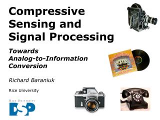
Compressive Sensing and Channel Coding: A Unified Perspective Amir H. Banihashemi BCWS Centre, Director Dept. of Systems and Computer Engineering Carleton University Ottawa, Canada JWCC 2010
Outline • Compressive Sensing • Channel Coding • Connections: Graphical Representation of Systems & Message-Passing Algorithms • Iterative Recovery Algorithms • Performance Analysis • Conclusion and Future Research JWCC 2010
Compressive Sensing[In part courtesy of R. Baraniuk, Rice University]
The Digital Universe • Size: 281 billion gigabytes generated in 2007 • digital bits > stars in the universe • growing by a factor of 10 every 5 years JWCC 2010
The Digital Universe • Size: 281 billion gigabytes generated in 2007 • digital bits > stars in the universe • growing by a factor of 10 every 5 years • Growth fueled by multimedia data • audio, images, video, surveillance cameras, sensor networks, … JWCC 2010
The Digital Universe • Size: 281 billion gigabytes generated in 2007 • digital bits > stars in the universe • growing by a factor of 10 every 5 years • Growth fueled by multimedia data • audio, images, video, surveillance cameras, sensor networks, … • In 2007 digital data generated > total storage JWCC 2010
The Digital Universe • Size: 281 billion gigabytes generated in 2007 • digital bits > stars in the universe • growing by a factor of 10 every 5 years • Growth fueled by multimedia data • audio, images, video, surveillance cameras, sensor networks, … • In 2007 digital data generated > total storage • Solution: Compression JWCC 2010
Why Compressive Sensing? • Problem: Today’s multimedia sensor systems acquire massive amounts of multimedia data only to throw much/most of it away. JWCC 2010
Why Compressive Sensing? • Problem: Today’s multimedia sensor systems acquire massive amounts of multimedia data only to throw much/most of it away. • Solution: compressive sensing JWCC 2010
Why Compressive Sensing? • Problem: Today’s multimedia sensor systems acquire massive amounts of multimedia data only to throw much/most of it away. • Solution: compressive sensing • - enables the design of radically new sensors and systems such as new cameras, imagers, ADCs, …, JWCC 2010
Why Compressive Sensing? • Problem: Today’s multimedia sensor systems acquire massive amounts of multimedia data only to throw much/most of it away. • Solution: compressive sensing • - enables the design of radically new sensors and systems such as new cameras, imagers, ADCs, …, • - beyond sensing to inference on massive data sets JWCC 2010
Digital Data Acquisition • Foundation:Shannon sampling theorem • “if you sample densely enough (at the Nyquist rate), you can perfectly reconstruct the original analog data” Space Time JWCC 2010
Sense by Sampling sample JWCC 2010
Sense by Sampling too much data! sample JWCC 2010
Sense (Sample) then Compress sample compress JPEG JPEG2000 … decompress JWCC 2010
Sparsity / Compressibility (Transform Coding) largewaveletcoefficients (blue = 0) pixels JWCC 2010
Sparsity / Compressibility (Transform Coding) largewaveletcoefficients (blue = 0) largeGabor (TF)coefficients pixels widebandsignalsamples frequency time JWCC 2010
What’s Wrong with this Picture? • Why go to all the work to acquire N samples only to discard all but K pieces of data? sample compress decompress JWCC 2010
Compressive Sensing • Directly acquire “compressed” data • Replace samples by more general “measurements” compressive sensing recover JWCC 2010
Sampling • Signal is -sparse in basis/dictionary • WLOG assume sparse in the canonical domain sparsesignal nonzero entries JWCC 2010
Sampling • Signal is -sparse in basis/dictionary • WLOG assume sparse in the canonical domain • Sampling (matrix multiplication) sparsesignal samples nonzeroentries JWCC 2010
Compressive Sampling • When data is sparse/compressible, one can directly acquire a condensed representation with no/little information loss through linear dimensionality reduction sparsesignal measurements nonzero entries JWCC 2010
How Can It Work? • In general, loss of information • Ex. Infinitely many ’s map to the same JWCC 2010
How Can It Work? • In general, loss of information • But we are only interested in sparse vectors columns JWCC 2010
How Can It Work? • In general, loss of information • But we are only interested in sparse vectors • is effectively M x K columns JWCC 2010
How Can It Work? • In general, loss of information • But we are only interested in sparse vectors • Design so that each of its M x K submatrices are full rank (ideally orthobases) columns JWCC 2010
How Can It Work? • Goal:Design so that for any K-sparse vector , norm of is “close” to norm of . [Restricted Isometry Property(RIP)] JWCC 2010
How Can It Work? • Goal:Design so that for any K-sparse vector , norm of is “close” to norm of . [Restricted Isometry Property(RIP)] • Unfortunately, this is NP-hard. JWCC 2010
How Can It Work? • Goal:Design so that for any K-sparse vector , norm of is “close” to norm of . [Restricted Isometry Property(RIP)] • Unfortunately, this is NP-hard. • Good news: Draw at random, e.g., i.i.d. Gaussian or i.i.d. Bernoulli. Then has the RIP with high probability provided JWCC 2010
Compressive Data Acquisition • Measurements = random linear combinations of the entries of • No information loss for sparse vectors with high probability sparsesignal measurements nonzero entries JWCC 2010
CS Signal Recovery • Goal: Recover signal from measurements JWCC 2010
CS Signal Recovery • Goal: Recover signal from measurements • Problem: ill-posed inverse problem JWCC 2010
CS Signal Recovery • Goal: Recover signal from measurements • Problem: ill-posed inverse problem • Solution: Exploit the sparse/compressiblenature of acquired signal JWCC 2010
CS Signal Recovery • Random projection • Recovery problem:givenfind • Null space • So search in null space for the “best” according to some criterion • ex: least squares (N-M)-dim hyperplaneat random angle JWCC 2010
CS Signal Recovery • Recovery: given(ill-posed inverse problem) find (sparse) • fast pseudoinverse JWCC 2010
CS Signal Recovery • Recovery: given(ill-posed inverse problem) find (sparse) • fast, wrong pseudoinverse JWCC 2010
CS Signal Recovery • Reconstruction/decoding: given(ill-posed inverse problem) find • fast, wrong number ofnonzeroentries “find sparsestin translated nullspace” JWCC 2010
CS Signal Recovery • Reconstruction/decoding: given(ill-posed inverse problem) find • fast, wrong • correct JWCC 2010
CS Signal Recovery • Reconstruction/decoding: given(ill-posed inverse problem) find • fast, wrong • correct slow: NP-hard JWCC 2010
CS Signal Recovery • Recovery: given(ill-posed inverse problem) find (sparse) • fast, wrong • correct, slow • correct, efficient mild oversampling[Candes, Romberg, Tao; Donoho]number of measurements required linear program JWCC 2010
“Single-Pixel” CS Camera scene single photon detector imagereconstructionorprocessing DMD DMD random pattern on DMD array w/ Kevin Kelly
“Single-Pixel” CS Camera scene single photon detector imagereconstructionorprocessing DMD DMD random pattern on DMD array … • Flip mirror array M times to acquire M measurements • Sparsity-based (linear programming) recovery JWCC 2010
Channel Coding • Essential in any communication link JWCC 2010
Channel Coding • Essential in any communication link • Advanced Coding Schemes: Turbo codes and low-density parity-check (LDPC) codes JWCC 2010
Channel Coding • Essential in any communication link • Advanced Coding Schemes: Turbo codes and low-density parity-check (LDPC) codes - Approach the capacity for many channels - Low-complexity iterative decoding algorithms - Excellent performance-complexity tradeoff JWCC 2010
Graphical Representation I II III • For linear block codes (including LDPC codes): Tanner Graph of (7,4) Hamming code I II III JWCC 2010
Iterative Decoding Algorithms Iterative decoding algorithms are “message-passing” algorithms in the graph Channel JWCC 2010
Iterative Decoding Algorithms Iterative decoding algorithms are “message-passing” algorithms in the graph JWCC 2010
Iterative Decoding Algorithms Iterative decoding algorithms are “message-passing” algorithms in the graph JWCC 2010