Steps in Statistical Testing:

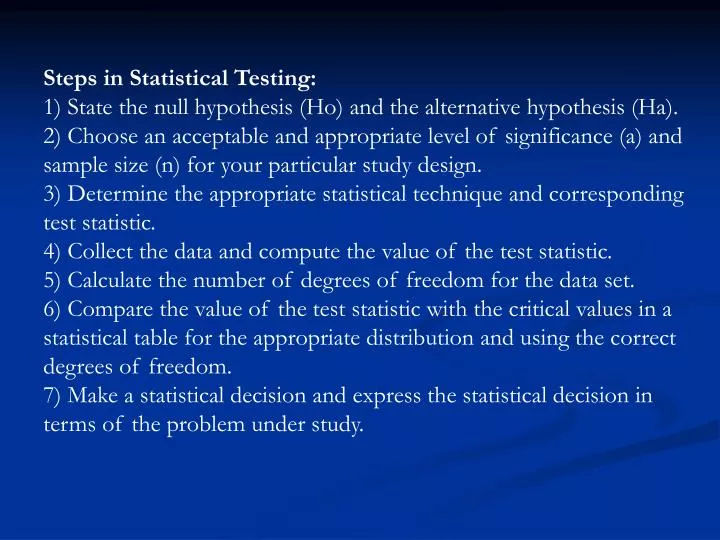
1. Steps in Statistical Testing: 1) State the null hypothesis (Ho) and the alternative hypothesis (Ha). 2) Choose an acceptable and appropriate level of significance (a) and sample size (n) for your particular study design. 3) Determine the appropriate statistical technique and corresponding test statistic. 4) Collect the data and compute the value of the test statistic. 5) Calculate the number of degrees of freedom for the data set. 6) Compare the value of the test statistic with the critical values in a statistical table for the appropriate distribution and using the correct degrees of freedom. 7) Make a statistical decision and express the statistical decision in terms of the problem under study.

2. P values • What is "statistical significance" (p-value). • The statistical significance of a result is the probability that the observed relationship (e.g., between variables) or a difference (e.g., between means) in a sample occurred by pure chance ("luck of the draw"), and that in the population from which the sample was drawn, no such relationship or differences exist. Using less technical terms, one could say that the statistical significance of a result tells us something about the degree to which the result is "true" (in the sense of being "representative of the population"). • Specifically, the p-value represents the probability of error that is involved in accepting our observed result as valid, that is, as "representative of the population." For example, a p-value of .05 (i.e.,1/20) indicates that there is a 5% probability that the relation between the variables found in our sample is a "fluke."

3. Why sample size matters • If there are very few observations, then there are also respectively few possible combinations of the values of the variables, and thus the probability of obtaining by chance a combination of those values indicative of a strong relation is relatively high. • Consider the following illustration. If we are interested in two variables (Gender: male/female and white cell count (WCC): high/low) and there are only four subjects in our sample (two males and two females), then the probability that we will find, purely by chance, a 100% relation between the two variables can be as high as one-eighth. • Specifically, there is a one-in-eight chance that both males will have a high WCC and both females a low WCC, or vice versa. Now consider the probability of obtaining such a perfect match by chance if our sample consisted of 100 subjects; the probability of obtaining such an outcome by chance would be practically zero.

4. sample size example • Example. "Baby boys to baby girls ratio." Consider the following example from research on statistical reasoning (Nisbett, et al., 1987). There are two hospitals: in the first one, 120 babies are born every day, in the other, only 12. On average, the ratio of baby boys to baby girls born every day in each hospital is 50/50. • However, one day, in one of those hospitals twice as many baby girls were born as baby boys. In which hospital was it more likely to happen? The answer is obvious for a statistician, but as research shows, not so obvious for a lay person: It is much more likely to happen in the small hospital. The reason for this is that technically speaking, the probability of a random deviation of a particular size (from the population mean), decreases with the increase in the sample size.

5. The number of degrees of freedom is the number of values in the final calculation of a statistic that are free to vary. Estimates of statistical parameters can be based upon different amounts of information or data. The number of independent pieces of information that go into the estimate of a parameter is called the degrees A data set contains a number of observations, say, n. They constitute n individual pieces of information. These pieces of information can be used to estimate either parameters or variability. In general, each item being estimated costs one degree of freedom. The remaining degrees of freedom are used to estimate variability. All we have to do is count properly. A single sample: There are n observations. There's one parameter (the mean) that needs to be estimated. That leaves n-1 degrees of freedom for estimating variability. Two samples: There are n1+n2 observations. There are two means to be estimated. That leaves n1+n2-2 degrees of freedom for estimating variability. One-way ANOVA with g groups: There are n1+..+ng observations. There are g means to be estimated. That leaves n1+..+ng-g degrees of freedom for estimating variability. This accounts for the denominator degrees of freedom for the F statistic. What are degrees of freedom?

6. Roadmap for next 5 weeks

7. Categorical Data Contingency table- examine the relationship between 2 categorical variables Chi Square Test McNemar’s Test- analysis of paired categorical variables, disagreement or change Mantel-Haenszel Test- relationship between 2 variables accounting for influence by a 3rd variable Parametric Alternatives Mann-Whitney U or KS- compare 2 independent groups, alternative to a t test Wilcoxon Sign Test- alternative to 1 sample t test Kruskal-Wallis- compare 2 or more independent groups alternative to ANOVA Friedman Test- compare 2 or more related groups alternative to repeated measures ANOVA Spearman’s Rho- association between 2 variables, alternative to pearson’s r Nonparametric Tests

8. Basic Methodology • Many nonparametric procedures are based on ranked data. Data are ranked by ordering them from lowest to highest and assigning them, in order, the integer values from 1 to the sample size. • Ties are resolved by assigning tied values the mean of the ranks they would have received if there were no ties, e.g., 117, 119, 119, 125, 128 becomes 1, 2.5, 2.5, 4, 5. (If the two 119s were not tied, they would have been assigned the ranks 2 and 3. The mean of 2 and 3 is 2.5.)

9. Contingency Table • Analyze the association between 2 categorical values • R possible responses x C possible categories • Uses counts (frequencies) in a crosstab table and perform Chi Square test • Chi square statistic compares observed counts with expected counts if there were no association • May combine categories before analysis to increase counts • Ho: There is no association between the 2 variables • Ha: the 2 variables are associated.

10. How is Pearsonian chi-square calculated for tabular data? • Calculation of this form of chi-square requires four steps: • Computing the expected frequencies. For each cell in the table, the expected frequency must be calculated. The expected frequency for a given column is the column total divided by n, the sample size. The expected frequency for a given row is the row total divided by n. The expected frequency for a cell is the column expectation times the row expectation times n. This formula reduces to the expected frequency for a given cell equaling its row total times its column total, divided by n. • Application of the chi-square formula. Let O be the observed value of each cell in a table. Let E be the expected value calculated in the previous step. For each cell, subtract E from O, then square the result and then divide by E. Do this for every cell and sum all the results. This is the chi-square value for the table. If Yates' correction for continuity is to be applied, due to cell counts below 5, the calculation is the same except for each cell, subtract an additional .5 from the difference of O - E, prior to squaring and then dividing by E. This reduces the size of the calculated chi-square value, making a finding of significance less likely -- a penalty deemed appropriate for tables with low counts in some cells.

11. Contingency Table General notation for a 2 x 2 contingency table. For a 2 x 2 contingency table the Chi Square statisticis calculated by the formula:

12. Table 2. Number of animals that survived a treatment. Contingency Table Results We now have our chi square statistic (x2 = 3.418), our predetermined alpha level of significalnce (0.05), and our degrees of freedom (df =1). Entering the Chi square distribution table with 1 degree of freedom and reading along the row we find our value of x2 (3.418) lies between 2.706 and 3.841. The corresponding probability is 0.10<P<0.05. This is below the conventionally accepted significance level of 0.05 or 5%, so the null hypothesis that the two distributions are the same is verified. Applying the formula above we get: Chi square = 105[(36)(25) - (14)(30)]2 / (50)(55)(39)(66) = 3.418 probability level (alpha)

13. McNemars Test • Paired values • before and after • Outcomes • + before and + after • + before and – after • - before and – after • - before and + after • Ho: The probability of a species having + before and – after is = to the probability of a species having – before and + after • Ha: The probability of a species having + before and – after is ≠ to the probability of a species having – before and + after

14. Mantel-Haenszel Comparison • Often used to pool results from multiple contingency tables • Detect influence of a third variable on 2 dichotomous variables • Ho: controlling for (or within forests) there is no relationship between dbh and tree age • Ha: controlling for (or within forests) there is a relationship between dbh and tree age

15. Mann Whitney U and Kruskal Wallis • 2 samples must be independent • Advantages over parametric t tests or ANOVA • Sample sizes are small and normality is questionable • Data contain extreme outliers • Data are ordinal • Ho: The groups have the same distribution • Ha: The groups do not have the same distribution • Kruskal Wallis • Ho: There are no differences in the distributions of the groups • Ha: There are differences in the distributions of the groups

16. To calculate the value of Mann-Whitney U test, we use the following formula: Where: U=Mann-Whitney U test N1=sample size one N2= Sample size two Ri = Rank of the sample size 1.      Arrange the data of both samples in a single series in ascending order. 2.      Assign rank to them in ascending order. In the case of a repeated value, assign ranks to them by averaging their rank position. 3.      Once this is complete, ranks of the different samples are separated and summed up as R1 R2 R3, etc. 4.      To calculate the value of Kruskal- Wallis test, apply the following formula: Where, H = Kruskal- Wallis test n = total number of observations in all samples Ri = Rank of the sample Mann Whitney and Kruskal Wallis

17. KW Example

18. Sign test and Wilcoxon Rank Sign • Paired values • Before and after • Stimulus and response • Counts number of positive and negative differences • WR Absolute values of differences Ho: The probability of a + difference is = to the probability of a – difference Ha: The probability of a + difference is ≠ to the probability of a – difference

19. Spearman’s Rho • Measures strength of an increasing or decreasing relationship between 2 variables • -1 to 1 • Advantages over Pearson’s r • Ranking procedure minimizes outliers • Ordinal data categories or ranges • Sample size is small or the normality of one of the variables is questionable