Download
1 / 29
290 likes | 466 Vues
BA203 Present Value Fundamentals. Richard Stanton Class 2, September 1, 2000. Topics Covered Last Class. Introduction to the language of the class Cash Flows Projects Firms Corporate Securities Common Stock (Equity) Preferred Shares Corporate Debt (Bonds). Overview of this class.

E N D
BA203Present Value Fundamentals Richard Stanton Class 2, September 1, 2000
Topics Covered Last Class • Introduction to the language of the class • Cash Flows • Projects • Firms • Corporate Securities • Common Stock (Equity) • Preferred Shares • Corporate Debt (Bonds)
Overview of this class • Evaluating individual investment projects • Use of Present Value (PV) • Role of capital markets in using PV • Role of consumption, borrowing, and lending with PV • Choosing among multiple projects • Investment opportunity curve • Maximizing PV as criterion for investment choice. • Optimal investment decisions
Overview • Evaluating individual investment projects • Use of Present Value (PV) • Role of capital markets in using PV • Role of consumption, borrowing, and lending with PV • Choosing among multiple projects • Investment opportunity curve • Maximizing PV as criterion for investment choice. • Optimal investment decisions
An Investment Decision • You can pay $3.5M today to construct a building in 1 year. • The interest rate “r” to borrow $3.5 M for 1 year is 10%. • The building will be will be worth $4.0 M next year. • Is it profitable to build this structure? • First attempt: $4.0M is bigger than $3.5M, so go ahead. What’s wrong with this answer? • The dates for construction cost and completed value differ • Need to compare them on a consistent basis • Convert the $4.0 M building value at date 1 to a present value, or • Convert the $3.5 M construction cost at date 0 to a future value. • We get the same result either way.
Applying Present Value (PV) and Future Value (FV) • Future value (FV) method: (C0 is $ borrowed) • FV of C0 = loan repayment amount = 3.5 x 1.10 = $3.85 • The building value (4.0) > FV of C0 (3.85), so do the project. • Present value (PV) method: (C1 is investment return) • PV of C1 = amount we need to invest today to have C1 next year. • PV = C1 / (1+r) = 4.0 / 1.1 = $3.64. • The PV ($3.64) > construction cost ($3.50), so do the project. • PV is generally computationally more convenient, especially when project investment returns cover a sequence of future periods
Net Present Value (NPV) • NPV = Project PV – Investment Cost • If Investment cost is $3.50 and PV = $3.64, then NPV= $3.64 - $3.50 = $.14 > 0 • General formula: NPV = C0 + C1/(1+r). • C0 is generally an investment cost, therefore negative. • NPV rule: Carry out project if NPV > 0. • Equivalently, the Rate of Return rule: Carry out project if return > r • In our example, return = (4.0 – 3.5) / 3.5 = 14.3% > 10%. • This rule makes intuitive sense, but when and why does it work?
More of both is better D B C Utility 3 Utility 2 Indifference A Utility 1 Indifference Curves $ Tomorrow (C1) - (Next year’s cash inflows) $ Today (C0) - (Money in the bank).
Prefers P2 Prefers P1 Project choice without capital markets
Project choicewithout capital markets • Mr. A prefers project 2. • Ms. B prefers project 1. Without knowing an investor’s consumption preferences, and absent a capital market, it is impossible to say one project is superior to another.
Slope of line is -(1 + r) Individual is lending in this range (less C0, more C1) Individual is borrowing in this range(more C0, less C1) The capital market budget line $ Tomorrow Initial position for individual (C0, C1) C1 C0 $ Today
2B 1B 2A (A lends) 1A(A borrows) PV of P2 PV of P1 Project choice with capital markets Still prefers P2 Also prefers P2 Project 2 has the higher PV
Present Value and Capital Markets • With a capital market all investors agree on the ranking of projects. • The highest Present Value (PV) project is best. • Thus, if an investment advisor only knows each project’s PV she can rank them for her clients.
Importance of Interest Rate At lower interest rate, both prefer Project 1
Consumption Shifting Exampler = 10% Project 1 Project 2
In general, PV = C0 + C1 / (1+r) Calculating Present Value • PV is what we consume today if we consume nothing next period. • For project 1, we need to borrow enough today that we pay back 20,000 next period. • Borrow 20,000 / 1.1 = 18,182. • So PV (Project 1) = 3,000 + 20,000 / 1.1 = 21,182 PV (Project 2) = 8,000 + 8,000 / 1.1 = 15,272
Overview • Evaluating individual investment projects • Use of Present Value (PV) • Role of capital markets in using PV • Role of consumption, borrowing, and lending with PV • Choosing among multiple projects • Investment opportunity curve • Maximizing PV as criterion for investment choice. • Optimal investment decisions
Choosing Among Many Projects • So far, we know that individuals rank projects according to their present value. • What about a firm, facing multiple possible investments, and with multiple different types of shareholder? • What rule should managers use in selecting projects?
Choosing Among Many Projects • You set up a firm whose assets are $1,000 in the bank and a corn farm. • Each row of corn costs $200 to seed. • There are 5 rows. • The payoff for each row is: • Row A: 50, B: 600, C: 400, D: 200, E: 100 • Plot the tradeoff between dividends today and dividends tomorrow.
A InvestmentOpportunityCurve E D C C: $200 cost, $400 crop B B: $200 cost, $600 crop $1000 in bank Planting Rows of Corn $ Tomorrow (slope tells usmarginal return) $ Today
Why is the Curve Concave? • Start all the way to the right. • The first $200 invested goes into the best project. • In our example, it yields $600 (row B) • The second $200 goes into the second best project. • In our example, it yields $400 (row C). • The third $200 goes into the third best project • It yields only $200 (row D), etc. • Continuing on, the curve gets flatter and flatter as you go to the left. • The marginal return gets smaller and smaller. • How far should we keep investing?
Investment Opportunity Curve • The investment opportunity curve reflects the firm’s ability to trade off dividends today (via forgone investment) for dividends tomorrow. • The slope of the curve represents the marginal return on the next dollar invested Fewer dividends today allows more dividends tomorrow More dividends today, means fewer tomorrow
Z is point of optimal investment. It has the highest PV, so allows the highest rate of consumption. Marginal return equals r. Worse off to invest either more or less. Budget line, slope –(1+r) Investment opportunity curve Marginal return is less than r. Better to invest less Marginal return is higher than r. Better to invest more. Total investment How many rowsshould you plant? Note: This does not depend on who the investors are
Firm’s Optimal Investment • Managers should thus • Take on every project with a return > r (positive NPV) • Reject every project with a return < r (negative NPV) • I.e. they should use the NPV rule. • This maximizes the PV of the firm. • All shareholders agree on this investment policy. • For alternative views of managers’ objectives, see Micro/OB • Note: the firm’s PV exceeds the cash it starts with. • Every time it invests in a +ve NPV project, the firm’s PV increases by the project’s NPV.
Total investment Firm’s Optimal Investment
What discount rate to use? • So far, we have assumed everything is riskless. • Our discount rate, r has been the riskless interest rate. • More generally, r represents the opportunity cost of capital. • The expected return available on other, “equivalently risky” investments. • We’ll see how to calculate this in the second half of the course • Idea: A project only makes us better off if its return is higher than the return we could get on alternative investments elsewhere. • NPV quantifies how much better off.
Summary of Lecture 2 • Choosing between two projects • Optimal choice with and without capital markets • Definition of Present Value (PV) • PV as criterion for investment choice by individual • Shifting consumption using borrowing and lending • Choosing among multiple projects • Investment opportunity curve • Maximizing PV as criterion for firm’s investment choice.
Course Resources for Lecture 2 • Brealey and Myers • Chapter 2 • Quiz, Practice Questions, Challenge Questions • Recommendations linked on web page • Answers in back of text, back of lecture reader. • Lecture Reader • Lecture 2. • Brealey and Myers Web site, http://www.mhhe.com/business/finance/bm/npv.mhtml
Preview of Lecture 3:The Present Value Formula • Brealey and Myers • Chapter 3 • Quiz, Practice Questions, Challenge Questions • Recommendations linked on web page • Answers in back of text, back of lecture reader. • Reader: Lecture 3 • Discussion case: for Wednesday 9/6.