Download
1 / 55
580 likes | 807 Vues
Chapter 4 Design Quality Estimation. Estimation. Estimates allow Evaluation of design quality Design space exploration Design model Represents degree of design detail computed Simple vs. complex models Issues for estimation Accuracy Speed Fidelity. Typical estimation model example.

E N D
Estimation • Estimates allow • Evaluation of design quality • Design space exploration • Design model • Represents degree of design detail computed • Simple vs. complex models • Issues for estimation • Accuracy • Speed • Fidelity
Accuracy vs. Speed • Accuracy: difference between estimated and actual value • Speed: computation time spent to obtain estimate • Simplified estimation models yield fast estimator but result in greater estimation error and less accuracy. |E(D)-M(D)| A=1- M(D) Estimation Error Computation Time Actual Design Simple Model
Fidelity • Estimates must predict quality metrics for different design alternatives • Fidelity: % of correct predictions for pairs of design Implementations • The higher fidelity of the estimation, the more likely that correct decisions will be made based on estimates. • Definition of fidelity: Metric estimate (A, B) = E(A) > E(B), M(A) < M(B) (B, C) = E(B) < E(C), M(B) > M(C) (A, C) = E(A) < E(C), M(A) < M(C) Fidelity = 33 % measured Design points A B C
Quality metrics • Performance Metrics • Clock cycle, control steps, execution time, communication rates • Cost Metrics • Hardware: manufacturing cost (area), packaging cost(pin) • Software: program size, data memory size • Other metrics • Power • Design for testability: Controllability and Observability • Design time • Time to market
Clock cycles metric • Selection of a clock cycle before synthesis will affect the practical execution time and the hardware resources. • Simple estimation of clock cycle is based on maximum-operator-delay method. • The estimation is simple but may lead to underutilization of the faster functional units. • Clock slack represents the portion of the clock cycle for which the functional unit is idle.
Clock slack and utilization • Slack: portion of clock cycle for which FU is idle slack ( clk , ti ) = ( [ delay ( ti ) / dk ] * dk ) – delay ( ti ) • Average slack: FU slack averaged over all operations ave_slack = • Clock utilization: % of clock cycle utilized for computations utilization=1 - T Σ [ occur (ti) * slack(clk,ti) ] i T Σ occur (ti) i ave_slack(clk) clk
Clock utilization 6x32 2x9 2 x 17 + + = 24.4 ns ave_slack(65 ns)= 6 + 2 + 2 utilization(65 ns) = 1 - (24.4 / 65.0) = 62%
Control steps estimation • Operations in the specification assigned to control step • Number of control steps reflects: • Execution time of design • Complexity of control unit • Techniques used to estimate the number of control steps in a behavior specified as straight-line code • Operator-use method. • Scheduling
Operator-use method • Easy to estimate the number of control steps given the resources of its implementation. • Number of control steps for each node can be calculated: • The total number of control steps for behavior B is
Operator-use method Example • Differential-equation example:
Scheduling • A scheduling technique is applied to the behavior description in order to determine the number of controls steps. • It’s quite expensive to obtain the estimate based on scheduling. • Resource-constrained vs time-constrained scheduling.
Scheduling for DSP algorithms • Scheduling: assigning nodes of DFG to control times • Resource allocations: assigning nodes of DFG to hardware(functional units) • High-level synthesis • Resource-constrained synthesis • Time-constrained synthesis
Classification of scheduling algorithms • Iterative/Constructive Scheduling Algorithms • As Soon As Possible Scheduling Algorithm(ASAP) • As Late As Possible Scheduling Algorithm(ALAP) • List-Scheduling Algorithms • Transformational Scheduling Algorithms • Force Directed Scheduling Algorithm • Iterative Loop Based Scheduling Algorithm • Other Heuristic Scheduling Algorithms
As Soon As Possible(ASAP) Scheduling Algorithm • Find minimum start times of each node
As Soon As Possible(ASAP) Scheduling Algorithm • The ASAP schedule for the 2nd-order differential equation
As Late As Possible(ALAP) Scheduling Algorithm • Find maximum start times of each node
As Late As Possible(ALAP) Scheduling Algorithm • The ALAP schedule for the 2nd-order differential equation
List-Scheduling Algorithm (resource-constrained) • A simple list-scheduling algorithm that prioritizes nodes by decreasing criticalness (e.g. scheduling range)
Force Directed Scheduling Algorithm (time-constrained) • Transformation algorithm
Force Directed Scheduling Algorithm • Figure.(a) shows the time frame of the example DFG and the associated probabilities (obtained using ALAP and ASAP). • Figure.(b) shows the DGs for the 2nd-order differential equation.
Force Directed Scheduling Algorithm • Example: Self_Force4(1) = Force4(1) + Force4(2) = (DGM(1)*x4(1)) + (DGM(2)*x4(2)) = (2.833*(1-0.5)) + (2.333*(0–0.5)) = (2.833*(+0.5)) + (2.333*(-0.5)) = +0.25
Force Directed Scheduling Algorithm • Example (con’d.): Self_Force4(2) = Force4(1) + Force4(2) = (DGM(1)*x4(1)) + (DGM(2)*x4(2)) = (2.833*(-0.5)) + (2.333*(+0.5)) = -0.25 Succ_Force4(2) = Self_Force8(2) +Self_Force8(3) = (DGM(2)*x8(2)) + (DGM(3)*x8(3)) = (2.333*(0-0.5)) + (0.833*(1–0.5)) = (2.333*(-0.5)) + (0.833*(0.5)) = -0.75 Force4(2) = Self_Force4(2) +Succ_Force4(2) = -0.25-0.75 = -1.00
A1 M2 A2 A3 M1 Force Directed Scheduling Algorithm(another example) A1: Fa1(0) = 0; A2: Fa2(1) = 0; A3: T(1): Self_Fa3(1)=1.5*0.5-0.5*0.5=0.5 Pred_Fm2(1)=0.5*0.5-0.5*0.5=0 Fa3(1) = 0.5 T(2): Self_Fa3(2)=-1.5*0.5+0.5*0.5=-0.5 Fa3(2) = -0.5 M1: Fm1(2) = 0; M2: T(0): Self_Fm2(0)=0.5*0.5-0.5*0.5=0 Fm2(0) = 0 T(1): Self_Fm2(1)=-0.5*0.5+0.5*0.5=0 Succ_Fa3(2)=-1.5*0.5+0.5*0.5=-0.5 Fm2(0) = -0.5
Scheduler • Critical path scheduler • Based on precedence graph (intra-iteration precedence constraints) • Overlapping scheduler • Allow iterations to overlap • Block schedule • Allow iterations to overlap • Allow different iterations to be assigned to different processors.
(2) B (2) (2) D A 2D C E (2) (1) Overlapping schedule • Example: • Minimum iteration period obtained from critical path scheduler is 8 t.u
Block schedule • Example: • Minimum iteration period obtained from critical path scheduler is 20 t.u 2D A B (4) (20)
Branching in behaviors • Control steps maybe shared across exclusive branches • sharing schedule: fewer states, status register • non-sharing schedule: more states, no status registers
Execution time estimation • Average start to finish time of behavior • Straight-line code behaviors • Behavior with branching • Estimate execution time for each basic block • Create control flow graph from basic blocks • Determine branching probabilities • Formulate equations for node frequencies • Solve set of equations
Probability-based flow analysis • Flow equations: freq(S)=1.0 freq(v1)=1.0 x freq(S) freq(v1)=1.0 x freq(v1) + 0.9 > freq(v5) freq(v2)=1.0 x freq(v2) freq(v3)=1.0 x freq(v3) freq(v4)=1.0 x freq(v3) + 1.0 > freq(v4) freq(v5)=1.0 x freq(v5) • Node execution frequencies: freq(v1)=1.0 freq(v2)=10.0 freq(v3)=5.0 freq(v4)=5.0 freq(v5)=10.0 freq(v6)=1.0 • Can be used to estimate number of accesses to variables, channels or procedures
Communication rate • Communication between concurrent behaviors (or processes) is usually represented as messages sent over an abstract channel. • Communication channel may be either explicitly specified in the description or created after system partitioning. • Average rate of a channel C, avgrate (C), is defined as the rate at which data is sent during the entire channel’s lifetime. • Peak rate of a channel, peakrate(C), is defined as the rate at which data is sent in a single message transfer.
Communication rate estimation • Total behavior execution time consists of • Computation time • Time required for behavior B to perform its internal computation. • Obtained by the flow-analysis method. • Communication time • Time spent by behavior to transfer data over the channel • Total bits transferred by the channel, • Channel average rate • Channel peak rate
56bits 1000ns Communication rates • Average channel rate rate of data transfer over lifetime of behavior averate (C ) = =56Mb/s • Peak channel rate rate of data transfer of single message peakrate(C ) = =80Mb/s 8bits 100ns
Area estimation • Two tasks: • Determining number and type of components required • Estimating component size for a specific technology (FSMD, gate arrays etc.) • Behavior implemented as a FSMD (finite state machine with datapath) • Datapath components: registers, functional units,multiplexers/buses • Control unit: state register, control logic, next-state logic • Area can be accessed from the following aspects: • Datapath component estimation • Control unit estimation • Layout area for a custom implementation
Clique-partitioning • Commonly used for determining datapath components • Let G = (V, E) be a graph,V and E are set of vertices and edges • Clique is a complete subgraph of G • Clique-partitioning • divides the vertices into a minimal number of cliques • each vertex in exactly one clique • One heuristic: maximum number of common neighbors • Two nodes with maximum number of common neighbors are merged • Edges to two nodes replaced by edges to merged node • Process repeated till no more nodes can be merged
Storage unit estimation • Variables used in the behavior are mapped to storage units like registers or memory. • Variables not used concurrently may be mapped to the same storage unit • Variables with non-overlappinglifetimes have an edge between their vertices. • Lifetime analysis is popularly used in DSP synthesis in order to reduce number of registers required.
Register Minimization Technique • Lifetime analysis is used for register minimization techniques in a DSP hardware. • A ‘data sample or variable’ is live from the time it is produced through the time it is consumed. After that it is dead. • Linear lifetime chart : Represents the lifetime of the variables in a linear fashion. • Note : Linear lifetime chart uses the convention that the variable is not live during the clock cycle when it is produced but live during the clock cycle when it is consumed.: • Due to the periodic nature of DSP programs the lifetime chart can be drawn for only one iteration to give an indication of the # of registers that are needed.
Lifetime Chart • For DSP programs with iteration period N • Let the # of live variables at time partitions n N be the # of live variables due to 0-th iteration at cycles n-kN for k 0. In the example, # of live variables at cycle 7 N (=6) is the sum of the # of live variables due to the 0-th iteration at cycles 7 and (7 - 16) = 1, which is 2 + 1 = 3. 3
i | f | c | h | e | b | g | d | a i | h | g | f | e | d | c | b | a Matrix Transposer Matrix transpose example • To make the system causal a latency of 4 is added to the difference so that Toutis the actual output time.
Circular Lifetime Chart • Useful to represent the periodic nature of the DSP programs. • In a circular lifetime chart of periodicity N, the point marked i (0 i N - 1) represents the time partition i and all time instances {(Nl + i)} where l is any non-negative integer. • For example : If N = 8, then time partition i = 3 represents time instances {3, 11, 19, …}. • Note : Variable produced during • time unit j and consumed during • time unit k is shown to be alive • from ‘j + 1’ to ‘k’. • The numbers in the bracket in • the adjacent figure correspond • to the # of live variables at each • time partition.
Forward-Backward Register Allocation Technique: Note : Hashing is done to avoid conflict during backward allocation.
Steps of Register Allocation • Determine the minimum number of registers using lifetime analysis. • Input each variable at the time step corresponding to the beginning of its lifetime. If multiple variables are input in a given cycle, these are allocated to multiple registers with preference given to the variable with the longest lifetime. • Each variable is allocated in a forward manner until it is dead or it reaches the last register. In forward allocation, if the register i holds the variable in the current cycle, then register i + 1 holds the same variable in the next cycle. If (i + 1)-th register is not free then use the first available forward register. • Being periodic the allocation repeats in each iteration, so hash out the register Rj for the cycle l + N if it holds a variable during cycle l. • For variables that reach the last register and are still alive, they are allocated in a backward manner on a first come first serve basis. • Repeat previous two steps until the allocation is complete.
Functional-unit and interconnect-unit estimation • Clique-partitioning can be applied • For determining the number of FU’s required, construct a graph where • Each operation in behavior represented by a vertex • Edge connects two vertices if corresponding operations assigned different control steps there exists an FU that can implement both operations • For determining the number of interconnect units, construct a graph where • Each connection between two units is represented by a vertex • Edge connects two vertices if corresponding connections are not used in same control step
Computing datapath area • Bit-sliced datapath