Download
1 / 50
500 likes | 790 Vues
The Deep Imaging Multi-Object Spectrograph for Keck II by S. M. Faber and the DEIMOS Team. Supported by CARA, UCO/Lick Observatory, and the National Science Foundation. Structural Overview. During Assembly. Final Assembly: Santa Cruz. At the Nasmyth Focus at Keck.

E N D
The Deep Imaging Multi-Object Spectrograph for Keck IIbyS. M. Faber and the DEIMOS Team Supported by CARA, UCO/Lick Observatory, and the National Science Foundation
Goals vs. Performance DEIMOS was conceived to be maximally efficient for faint-object spectroscopy of objects densely packed on sky • Minimize the effect of sky background • “Get between” OH lines: =1.25 A, R = 6000 , x4 speed gain • Accurate flat-fielding: 0.2% rms (photon-limited for 10-hr exposures) • Stable image position (fringing): 0.6px rms(goal) • High observing efficiency • Long slit length on sky: 16.7’, >130 slitlets • Broad spectral coverage: 2000 resolution elements • High throughput: 28% peak (with atm & tel; 50% DEIMOS alone) • Low readout noise: 2.3 e– • Fast readout time: 50 sec • Rapid slitmask alignment: 5 min(goal) • Excellent image quality (3800 A to 10,500 A) • Hoped for: 0.6-0.8 px (1-d rms with 15 pixels) • Actual: 0.8-1.2 px => ~2.0-2.8 px FWHM
Detector Performance The detector is a mosaic of 8 2K x 4K CCDs from MIT/Lincoln Laboratories. The CCDs are high-resistivity, red-sensitive devices that are 45 thick, with a peak QE of 85% and enhanced QE of 23% at 10,000 A.
DEIMOS Masksand Detector • Slit masks are curved to match the focal plane and imaged onto an array of 2k 4k CCDs • Readout time for full array (150 MB!) is 50 seconds (8 amplifier mode)
4 px FWHM 8000px 800px Arc Spectrum: 133 slitlets
S II under OHline z= 0.19 Sky-subtracted Sub-regions
S II under O2 band z = 0.28 Sky-subtracted Sub-regions
S II at z = 0.075 6 e– peak cts Sky-subtracted Sub-regions
Vrot ~100 km/s z = 0.90 Vrot ~100 km/s z = 0.92 Kinematic Information
O II at z = 1.29 vrot ~ 100 km/s Kinematic Information
O II at z = 0.80 < 30 km/s Kinematic Information
O III 5007/4959 at z = 0.62 v = 680 km/s Kinematic Information
Sky Subtraction is Key Left:Raw data from an unaligned DEIMOS slitmask, with serendip (detail). Some slitlets are tilted to allow rotation curve measurements; this poses unique challenges for automated sky subtraction. Below:test analysis of one tilted slitlet. From top: raw data, b-spline model of the night sky lines, and rescaled residual. We already can achieve sky subtraction at close to the Poisson limit in cases like this.
Typical Extracted 1-d Spectrum Unsmoothed 1-d spectrum with background sky (red) offset and rescaled.
Poisson-Limited Sky Subtraction Plot shows residual of flux from b-spline sky model in region of sky emission lines, in units of local RMS. Smooth curve is gaussian, width 1. Work in progress todo non-local sky subtraction using narrower, sky-only slitlets, for the shortest slitlets where local sky subtraction is impossible.
The UCB Automated Data Pipeline A small group of galaxies with velocity dispersion 250 km/s at z 1. Note the clean residuals of sky lines.
CCD Crosstalk • The image from CCD 6 appears negatively on CCD5 • The amplitude saturates at about 2.5 e– • The main effect is to create negative sky lines. The widths depend on line brightness unpredictably • Possibly due to open wire on CCD5 A amplifier • Action is TBD
Optical Performance The camera was designed by Harland Epps. It has exceedingly wide field of view (11.4° radius), three steep aspherics, three large CaF2 elements, a passive thermal plate-scale compensator, and three fluid-coupled multiplets.
14 in diam! Camera/Dewar Layout
Images at First Assembly Radial comatic tails, max 15 px
Causes of Radial Coma • Inherent in optical design: performance at room temperature differs from 0 C Accounts for about half of effect • Element 8/9 spacing too short • Detector too deep in dewar • Multiplet 4 slightly too thick
El 8/9 spacing Detector tilt X,Y lateral adjustment screws Three Optical Adjustments
Sample Images: Dome Lights Detectorcenter Line profile Image: 0.5” pinholes
Line Profiles: Top, Center, Bottom Bottom Top Center No coma Nocoma
Measured Image Sizes • Estimated RMS image sizes, corrected for 0.5” pinhole ActualPredicted Center Corners Center Corners 1-d : 0.88 px 1.17 px 0.60 px 0.82 px 13.2 17.5 8.8 12.0 FWHM: 2.07 px 2.75 px 1.41 px 1.93 px 31.7 41.2 21.1 px 29.0 • Extra source of broadening equivalent to 11.3 (1-d ) • Possibility: refractive index inhomogeneities? CaF2?
Image Stability The original passive specification for image motion was 6 px peak-peak under 360 rotation in X and Y. This goal has not been met, but the final image stability specifications seem to be within reach nevertheless.
Image Stability/Flexure • Reasons for wanting stable images • Image quality X is along slit • Needed during single exposure Y is along spectrum • Affects both X and Y • Specification: < 1 px rms • Flat-fielding accuracy • Needed between afternoon calibrations and evening observations • Flat-fielding accuracy requirement: 0.2% rms • Affects Y only (along spectrum) • Specification: < 0.6 px rms (originally 0.25 px rms) • Use flat fields to delineate slitlet edges • Needed between afternoon calibrations and evening observations • Affects X only (across spectrum) • Specification: < 1 px rms
Flexure Compensation System • Closed feedback loop: both centroid sensing and correcting • Operates in both direct imaging and spectroscopy modes • Sensing system • Four optical fibers pipe CuAr light (or LED) into telescope focal plane at opposite ends of slitmask • Two separate sensing CCDs are mounted on detector backplane flanking the science mosaic • These FCS CCDs are read every 40 sec when shutter is open • Feedback is achieved only when shutter is open • Correcting system • Steers image in X and Y; no rotation • X actuator: motor in dewar moves detector along slit • Y actuator: piezo on tent mirror moves spectrum in
X actuator: on detector Y actuator: on tent mirror FCS Actuators
Flexure History • Initial image motion on first assembly: X motion: 40 px Correctable range: 26 px Y motion: 7 px 13-23 px MUST FIX X MOTION! • Year-long campaign discovered moving elements in camera and grating system • Current image motion: X motion: 8 px Y motion: 18-23 px (depends on grating or mirror) • Lessening X increased Y to some degree • Tilting grating is needed in Y in addition to tent mirror
Y X Y Correction: First Results • Performance with closed-loop correction • Total image motion through 360° rotation, in px; slider 3; USING ONLY ONE FIBER ON ONE FCS • Nature of motion: sag in Y, larger with X (i.e., a shear) • Probable cause: pitch of collimator • Expectation: final rms will be 0.4-0.5 px …. meets goal 0.75 1.00 1.62 RMS = 1.0 px Y motions 0.31 0.75 1.25 RMS resid= 0.4 px 0.50 1.25 1.19 Goal = 0.6 px Position on detector
Y X X Correction: First Results • Performance with closed-loop correction • TOTAL image motion through 360° rotation, in px; slider 3; USING ONLY ONE FIBER ON ONE FCS • Nature of motion: shift in X, mainly bulk motion • Probable cause: flexure in the fiber mount • Expectation: final rms will be 0.6-0.7 px …. meets goal 2.43 2.25 2.88 RMS = 2.1 px X motions 1.62 2.38 2.00 RMS resid= 0.5 px 1.25 2.13 1.95 Goal = 1.0 px Position on detector
Lessons Learned • “Success-oriented” does not work at this scale • Expect that most mechanisms will NOT work as designed the first time. Hence… • Build prototypes and test extensively before putting into spectrograph • The major source of flexure is not the main structure but rather mechanisms attached to the structure; not easily analyzed using FEA; hence the need for prototypes
Final Lesson: Naming Phobos and Deimos were the horses that pulled the chariot of Aries, the god of war. • Phobos means “fear.” • Deimos means “the awe one feels on the battlefield when in the presence of something greater than oneself.” MORAL: be careful naming your instrument; names have a way of coming true
Comparison Between DEEP2 1HS and Local Surveys SDSS 2dF LCRS DEEP2 z~0 CFA+SSRS PSCZ z~1
Colors Pre-select Distant Galaxies • Plotted at left are the colors of galaxies with known redshifts in our fields; those at low redshift are plotted as blue, those at high redshift as red(diamonds are beyond the mag. limit of the survey). • A simple color-cut defined by three line segments would yield a sample >90% at z>0.75 and missing <3% of the high-z objects. Most of the failures are likely to be due to photometric errors.
Test of Photo-z Selection Procedure Redshift distributions in early masks are consistent with expectations
Simulated DEEP2 Spatial Sampling Courtesy A. Coil Targeted objects are included when our slitlet assignment algorithm is performed on a mock DEEP2 survey created from an N-body simulation; missed objects are those not selected
Another Redshift Survey: The VLT/VIRMOS Project • 50,000 galaxies to IAB< 24 (1.2 sq. deg) • 105 galaxies with IAB< 22.5 (9 sq. deg) • 750 simultaneous slitlets (4 barreled instrument) • Resolution R~ 180-2520: short spectra, multiple spectra per row • 100+ nights on VLT-3: Observations start November 2002
Property DEEP2 VLT/VIRMOS Survey Size 65000+6500 130,000+50,000+3000 Multiplexing 120-140 galaxies 750 galaxies Resolution R=/ 5000 200 200 2500 Wavelength Range ~2600 Å ~2500 Å Magnitude Limit IAB< 23.5 – 24.5 IAB< 22.5 – 24 Redshift Range 0.7 < z < 1.4 0<z<? Only half with z >0.7 0-order Summary LCRS at z~1 CFRS for the 21st century DEEP2 versus VLT/VIRMOS HAS VIRMOS chosen quantity over quality? • Only half their galaxies will be distant • Most of their galaxies have resolution 200, not 5000; no kinematic info; inferior velocities? • They cannot subtract sky accurately at R=200; will lose x2 overhead for “nod and shuffle”
Advantages of DEEP2 over VLT/VIRMOS • Higher resolution: • Provides more precise redshifts and allows secure z measurements from the [OII] doublet alone • Permits us to measure linewidths/rotation curves • Reduces contamination by night skylines • Necessary for many of our science goals: e.g. T-F type relations, studies of bias (e.g. via redshift-space distortions), measurement of thermal motions, determining velocity dispersions of clusters, the dN/dz test… None of these will be possible with low-resolution VLT/VIRMOS data. • Photometric cut for z>0.7 will eliminate ~50% of all galaxies with IAB< 23.5from target list, yielding denser sampling at z ~1
Schedule of the DEEP2 Survey • DEIMOS has been reassembled and tested at Mauna Kea • Commissioning began June 2002 under clear skies and was extremely successful • DEEP2 observing campaign began in July 2002. (so far we have had 4:9 science nights clear, and on 3:4 of these, the TV camera was broken!) • Observations complete late 2004 (we hope) • Analysis complete late 2006