Download
1 / 20
200 likes | 305 Vues
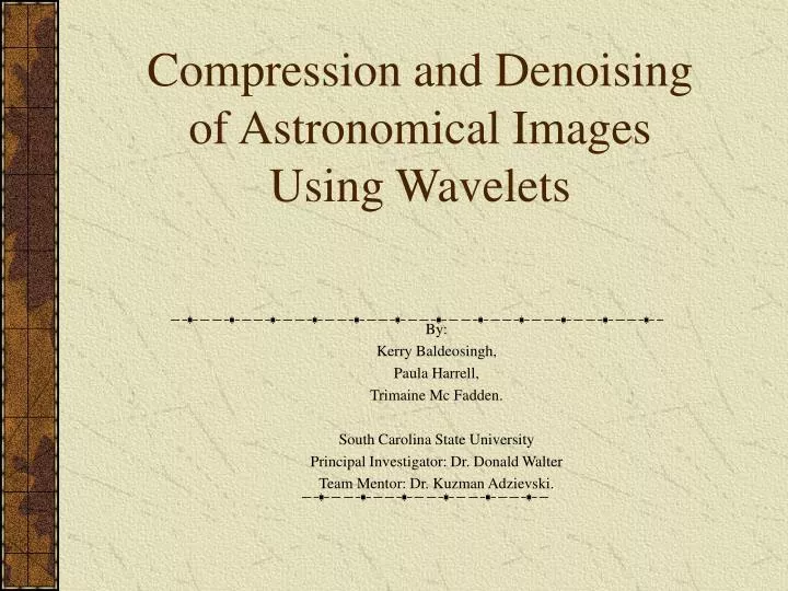
Compression and Denoising of Astronomical Images Using Wavelets. By: Kerry Baldeosingh, Paula Harrell, Trimaine Mc Fadden. South Carolina State University Principal Investigator: Dr. Donald Walter Team Mentor: Dr. Kuzman Adzievski. Outline. Wavelets and some of their applications .

E N D
Compression and Denoising of Astronomical Images Using Wavelets By: Kerry Baldeosingh, Paula Harrell, Trimaine Mc Fadden. South Carolina State University Principal Investigator: Dr. Donald Walter Team Mentor: Dr. Kuzman Adzievski.
Outline • Wavelets and some of their applications. • Haar and Daubechies wavelets. • Compression and Denoising. • Summary and results of image denoising.
What are wavelets? • Wavelets are functions that are generated from one single function, known as the mother wavelet.
Applications of Wavelets • Wavelets are used in many fields: physics, astronomy, mathematics, biomedicine, computer graphics. • In our paper we use wavelets for compression and denoising of astronomical images.
Discrete signals and images • A discrete signal is a function f with values at discrete instances and usually it is expressed in the form: f = ( f1, f2, f3, f4, f5, f6, … fN-1, fN ). • A discrete image, f, is an array of M rows and N columns and is expressed in the form: f =
Types of Wavelets • Haar • Daubechies • Coiflets
Haar Wavelets • The Haar wavelet is the simplest type of wavelet. • They are related to a mathematical operation called the Haar transform which serves as the model for other wavelet transforms.
Haar Transform • A 1D, 1-level Haar transform is performed on a signal, f = ( f1, f2, f3, f4,… fN-1, fN ), is f( a1| d1 ) where a1= (f1 + f2 )/ √(2) , (f3 + f4 )/ √(2),… and d1 = (f1 – f2 )/ √(2), (f3 – f4 )/ √(2),… • a1 is called the trend or running average. d1is called the fluctuation or running difference. • This process can be repeated until there ceases to be an even number of averages. • Performing an inverse transform only to the trend sub signal would allow an approximation of the original signal.
Daubechies Wavelets and transforms • There are various types of Daubechies transforms. We use the Daub4 transform which is slightly more complex than the Haar transform.
Daub4 transform • This Daub4 transform involves using constant values α1, α2, α3 and α4 and β1, β2, β3 and β4 which are found from solving a set of equations. • If a signal f = ( f1, f2, f3, f4, f5, f6, … fN-1, fN ), then a 1D, 1-level transform will be: f( a1| d1 ) where a1 = (α1f1 + α2f2 + α3f3 + α4f4 ), (α1f3 + α2f4 + α3f5 + α4f6 ), …(α1fn-1 + α2fn + α3f1 + α4f2 ) d1 = (β 1f1 + β 2f2 + β 3f3 + β 4f4 ), (β 1f3 + β 2f4 + β 3f5 + β 4f6 ),… (β 1fn-1 + β 2fn + β 3f1 + β 4f2 ) • A 1D 2-level transform would be f(a2| d2 | d1)
2D Wavelet transform • A 2D wavelet transform of a discrete image can be performed only when the image has an even number of rows and columns. • A 1-level wavelet transform of an image involves: • A 1D, 1-level, wavelet transform on each row of the image, producing a new image. • Then on the new image, a 1D, 1-level wavelet transform is performed on each of its columns. • If f is an N x M, 2D array of an image, then under a 1-level wavelet transform f can be symbolized as:
2D Wavelet transform • From an image f: • a1 = trend rows then trend columns. • h1 = trend rows then fluctuation columns. • d1 = fluctuation rows then fluctuations columns. • v1 = fluctuation rows then trend columns. • A 2D 2-level transform is calculated by computing a 1-level transform of the trend subimage a1:
Compression • Compression relies on converting data into a smaller format that allows the transmission of fewer bits. • There are two types of compression: • Lossless • No image data is lost as a result of compression. • No errors in result. • Compression ratios of up to 2:1 can be obtained. • Lossy • Some image data is lost as a result of compression. • Results have small inaccuracies. • Compression ratios of up to 100:1 can be obtained.
Method of compression • The basic steps of compression are as follows: • Perform a wavelet transform of the signal. • Set equal to 0 all values of the wavelets transform which are insignificant, i.e., which lie below some threshold value. • Transmit only the significant, non-zero values of the transform obtained from Step. 2. This should be a much smaller data set than the original signal. • At the receiving end, perform the inverse wavelet transform of the data transmitted in Step. 3, assigning zero values to the insignificant values which were not transmitted. This decompression step produces an approximation of the original signal.
Denoising Gaussian noise • Find the mean, μ, and the standard deviation, σ, of the image. • The image is then transformed once. • Using the value of the standard deviation, σ, a thresholding value, T, can be established where T = 4.5 σ. • Approximately 99% of the noise can be removed. • Success of this method depends on how well the transform compresses the signal into a few high magnitude values that stand out.
Soft and Hard thresholdiing • Hard thresholding: • Soft thresholding • In hard thresholding, the transform is not continuous and thus those values near the threshold are greatly exaggerated. In soft thresholding the function does not abruptly change thus an inverse transform from soft thresholded values produce a better quality denoised image.
Results Image with random noise
Coif 6 (denoise) Level 1 Threshold 150.965 Avg. 2 Daub 20 (denoise) Level 1 Threshold 213.4967 Avg. 4 Coif 6 (series) Level 1 3611 coefficients used, 22.%. Threshold: 1/2^2 Bits per pixel: 0.66 Daub 20 (series) Level 1 3625 coefficients used, 22.1%. Threshold: 1/2^2 Bits per pixel: 0.66 Denoised Images 1
Daub 20 (denoise) Level 1 Threshold 213.4967 Avg. 8 Haar (denoise) Level 1 Threshold 213.4967 Avg. 1 Daub 12 (series) Level 1 1159 coefficients used, 7.1%. Threshold: 1/2^1 Bits per pixel: 0.14 Haar (series) Level 1 5225 coefficients used, 31.9%. Threshold: 1/2^3 Denoised Images 2
References and useful tools • Walker S. James. Wavelets and their Scientific Applications, A Primer. CRC Press LLC, Boca Raton, Florida, 1999. • http://www.crcpress.com/edp/download. FAWAV Software for Wavelet Analysis • Mathematica Software Package, Wolfram Research Inc. • Dr. Kuzman Adzievski. In-class Lectures and Recitations. • http://hubble.stsci.edu/gallery/showcase/stars/s1.html. Globular Cluster M80 • Acknowledgement: I would like to thank Dr. Daniel Smith for the helping me loading the JPEG images using the Mathematica software.