Download
1 / 29
290 likes | 388 Vues
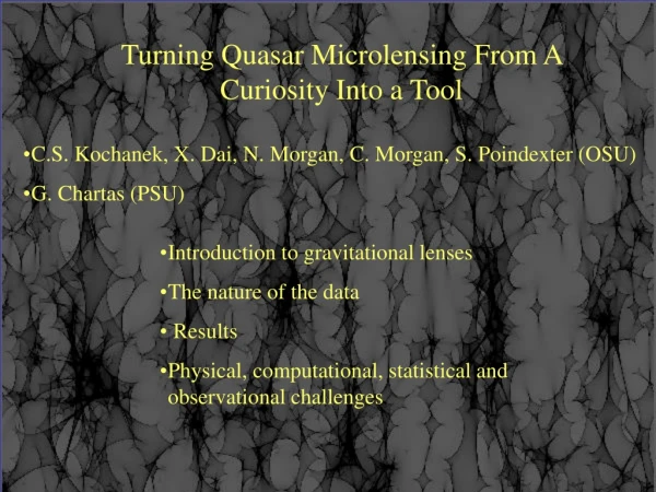
Turning Quasar Microlensing From A Curiosity Into a Tool. C.S. Kochanek, X. Dai, N. Morgan, C. Morgan, S. Poindexter (OSU) G. Chartas (PSU). Introduction to gravitational lenses The nature of the data Results Physical, computational, statistical and observational challenges.

E N D
Turning Quasar Microlensing From A Curiosity Into a Tool • C.S. Kochanek, X. Dai, N. Morgan, C. Morgan, S. Poindexter (OSU) • G. Chartas (PSU) • Introduction to gravitational lenses • The nature of the data • Results • Physical, computational, statistical and observational challenges
The Gravitational Lens RXJ1131-1231 Quasar image D Quasar image B “Einstein Ring” image of quasar host galaxy Quasar image A Quasar image C lens galaxy
Monitor Quasar Image Brightness • Two sources of time variability • Intrinsic quasar variations, which appear with a “time” delay between each image • Uncorrelated variations due to “microlensing” by the stars in the lens galaxy (For non-astronomers, magnitudes are –2.5log(flux)+constant)
First Determine Time Delays • For RXJ1131-1231 they are +12, +10 and –87 days for images B, C and D relative to A (B leads, D trails) • The delays can be used to study the mass distribution of the lens or to estimate the Hubble constant, but this is not our present topic
What’s left is the “microlensing”: Variations in the flux ratios of the images after correcting for the time delays
What Determines an Image’s Flux? • The local magnification is determined by the local derivatives of the potential, • What contributes to these derivatives? • Overall smooth potential – the “macro” model • Satellites/CDM substructure – millilensing • Stars – microlensing • Finite source sizes smoothing of the small scale structures in the magnifications, in particular, smoothing of the caustics on which the magnification diverges
Length Scales Set by the mass of the lenses and the distances • Lens galaxy M~1010M• E~1arcsec • Satellite galaxy M~106M• E~10 milliarcsec • Star M~M• E~10 microarcsec The stars produce complex magnification patterns with different structures near each image
Source plane scale=40<E> 2h-1<M/M•>1/2pc=335<M/M•>1/2as B C D A For a 109M• black hole RBH=0.0001pc =0.01as =0.l<M/M•>-1/2pixels
What can we study using microlensing? • Quasar Structure – microlensing “resolves” quasar accretion disks, allowing us to measure their structure as a function of wavelength • Dark matter – microlensing depends on the fraction of the mass near the lensed images comprised of stars • Stellar populations – microlensing can estimate the mean stellar mass the halos of cosmologically distant galaxies
Quasar Accretion Disks Have A Very Similar Size Scale Should be able to study structure of quasar accretion disks because variability amplitude source size
Minima Saddle Points Depends on the fraction of the surface density in stars High optical depth Low optical depth Or in the statistics (Schechter & Wambsganss 2002)
Mean Stellar Mass • All “observable” properties of the microlensing are in “Einstein units” of <M/M>1/2cm. Converting to just cm requires a prior on • The mean microlens mass <M> • The true physical velocities • The true source size • We have good physical priors for the physical velocities, which means we can sensibly estimate <M> in cosmological distant galaxies
But how do you go from light curves to physics? One of the two basic problems in using quasar microlensing for astrophysics. The other is the sociological difficulty of doing the observations. OGLE (Wozniak et al. 2000ab) microlensing light curves of Q2237+0305
For Galactic microlensing events you just fit the light curves. Binary microlensing event MACHO 98-SMC-1 In this case solutions must include binary orbital motion….. Afonso et al. 2000
We will just do the same, using computer power and the Reverend Bayes • Given the local properties (, *, ) and the stellar mass function • Generate random realizations of the magnification patterns • Given a model for the quasar accretion disk • Randomly choose disk parameters, convolve with patterns • Given a random selection of a source velocity • Randomly pick nuisance parameters (direction, starting point) • Fit the resulting light curve to data to estimate a 2 statistic • Combine all the trials using Bayesian methods to estimate probability distributions for the values of interesting parameters
We Obtain Statistically Acceptable Fits To The Data Good fits mean fitting all 6 difference light curves between the 4 images (the average light curve gives the intrinsic source variability)
Are Galaxies Composed of Stars? Q2237+0305 RXJ1131-1231 Most lenses, like RXJ1131-1231, should only have a small fraction of the surface density near the quasar images comprised of stars (/*~0.1 to 0.2), but one lens, Q2237+0305, where we see the images through the bulge of a low redshift spiral galaxy, should be almost all stars (/*~1)
The Microlensing Knows….. (although for most lenses it has yet to converge significantly) RXJ1131-1231 should be mostly dark matter Q2237+030 should be mostly stars
What is Mean Mass of the Microlenses? All directly measured quantities are in “Einstein units” <M>1/2cm Best physical priors are for the true velocities P(ve) Q2237+030 • For any one lens, the uncertainties will be large: • Mass goes as (velocity)2 • Physical prior for any one less has a velocity uncertainty of order a factor of two from the unknown peculiar velocity Best single case Q2237+0305 <M> = 0.61 M 0.12 M <M> 2.85 M
Ensembles of Lens Should Provide An Accurate Estimate • Dominant uncertainty in priors is a random variable (peculiar velocities) whose dispersion is known, but not the value for a particular system • Multiply P(<M>) for each system to get a joint estimate for ensemble of lenses • Must hit a systematic floor at some point, but almost certainly not yet Combining the 8 systems (mostly) analyzed as of Saturday… <M> = 0.09 M 0.04 M <M> 0.19 M Answer stable to dropping any one lens, but it would be nice to see the outliers shift towards the median as we accumulate longer light curves.
Disk Scale Lengths Well-Determined Why? Because the mass scale uncertainties affect the source size little Means that the physical source size is little affected by the uncertainties in the mass, which is very convenient!
Beginning to Test Accretion Disk Theory Black hole masses estimated from emission line-width/mass correlations
Disk Structure Best Probed As Size Versus Wavelength First tests, surprisingly, are optical versus X-ray sizes CXO Spring 2004 CXO Spring 2006 Blackburne et al OSU/PSU • Optical and X-ray flux ratios very different, and change differently with time (now known for 4 lenses) • Smaller sources will show greater microlensing variability
Partial results for 3 systems now, additional data being collected, but X-ray sources are roughly 1/10 the size of the optical sources As expected, size ratios are less uncertain than absolute sizes (remember, the X-ray size is being determined from 4 data points!)
Issues of Physics • Mass function of microlenses – extensive prior theoretical studies showing that this is very hard to probe and has little effect on results • Disk structure at fixed wavelength – extensive prior theoretical studies show that microlensing data measures typical size rather than details of the surface brightness distribution – better to focus on size versus wavelength, black hole mass etc.. • Only time variability or also observed flux ratios – observed flux ratios are also affected by substructure (satellites) and extinction/absorption, but they are powerful constraints on where you sit in the microlensing magnification pattern • The stars move. Except in experiments, we have used fixed magnification patterns, but in real life they change with time as the stars move. Theoretical studies suggest that we are safe so far, but not forever.
Issues of Computation • With some physically irrelevant fiddles, it is possible to make the image and source regions periodic – allows use of FFTs to generate magnification patterns and leads to periodic magnification patterns that simplify the Bayesian analysis method • Dynamic range of magnification patterns – need to maintain a large enough outer scale to get a fair sample of stars, and a small enough inner scale to deal with compact sources – 40962 maps marginally OK • Computationally challenging to allow stars to move – we need ~3 GByte to analyze a systems at 2 wavelengths with static patterns, but ~300 GBytes if we allow the stars to move and need an animated sequence of patterns. Probably doable on shared memory machines (and we have experimented with this), but could lead to catastrophic time penalties on other parallel machines because of the need for random access to all the patterns (awaits a really good computational student). • Fiddles to speed execution. We have incorporated various fiddles to make the analysis run FAST. The most serious of which is an inner loop that does a local maximum likelihood search over nuisance variables that is not strictly in accordance with the Bayesian outline of the calculations. • Monte Carlo verification. We need to spend more effort on generating fake data sets and verifying that the analysis performs as expected. So far, so good, but….
Issues of Statistics • All looks pretty good, except for: • The interaction of priors, static magnification maps and the reality that the stars move and we need to animate the maps – current approach does not do this properly but is designed (hopefully!) to lead to overly broad uncertainty estimates on the physically interesting quantities • The inner, hidden, maximum likelihood loops where we allow a local optimization of the nuisance variables over restricted ranges. Needs more study to better approximate the true Bayesian integrals • Stratified/likelihood sampling of physical variables needs to be understood/implemented to minimize wasted time on low likelihood regions of parameter space • Testing with simulated data needs to be massively expanded
Issues of Observation • Obtaining the necessary observations remains our biggest problem • We monitor ~20 lenses well at at one wavelength (R band), with lesser coverage at J, I and B • The Babylonian observer problem for ground based optical/near-IR remains a major problem. For example, all our results are for lenses visible from the queue-scheduled SMARTS telescope at CTIO – we cannot do similar analyses for Northern lenses. • To study how the region near the last stable orbit differs from regions further from the last stable orbit, we need UV observations with HST – success depends on obtaining long (years) time baselines before HST fails. No luck so far …. • To study the X-ray emitting region at “low resolution” we need continued support for short (<10ksec) CXO observations – measurement accuracy largely depends on having reasonable sampling over long temporal baselines. Good luck so far…. • To study the X-ray emitting region at “high resolution,” meaning the relative sizes of the hard, soft and X-ray line emitting regions, will require a major effort (~100 ksec exposure times). Hopefully, we prove our method with the current observations, propose and get shot down next year, propose and succeed the following….. • On the plus side, this is much better than we achieved in the proceeding 20 years, during which we completely wasted the opportunity to do this physics because of the sociological barriers!
Summary • We are achieving physical interesting results that no one expected from this approach. We can estimate • The surface density of stars relative to dark matter • The average mass of the stars • The structure of the accretion disk as a function of wavelength • All of which are new and unique probes of great astrophysical relevance • We are primarily data limited at the present time given the ability to collect the necessary data, we can dramatically improve over our already completely unexpected results • There are challenging computational and statistical issues if we can get that data