Download
1 / 19
200 likes | 329 Vues
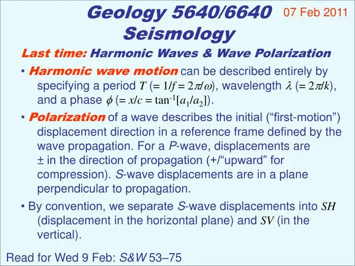
Geology 5640/6640 Seismology. 07 Feb 2011. Last time: Harmonic Waves & Wave Polarization Harmonic wave motion can be described entirely by specifying a period T ( = 1/ f = 2 / ), wavelength ( = 2 / k ), and a phase ( = x / c = tan -1 [ a 1 / a 2 ] ).

E N D
Geology 5640/6640 Seismology 07 Feb 2011 • Last time:Harmonic Waves & Wave Polarization • Harmonic wave motion can be described entirely by • specifying a period T (= 1/f = 2/), wavelength (= 2/k), • and a phase (= x/c = tan-1[a1/a2]). • Polarization of a wave describes the initial (“first-motion”) • displacement direction in a reference frame defined by the • wave propagation. For a P-wave, displacements are • ± in the direction of propagation (+/“upward” for • compression). S-wave displacements are in a plane • perpendicular to propagation. • • By convention, we separate S-wave displacements into SH • (displacement in the horizontal plane) and SV (in the • vertical). Read for Wed 9 Feb: S&W 53–75
Seismic Data and Analysis: First, a quick look at some data and phases
Ray Naming Conventions P, S - P or S wave segments in the mantle p, s - up-going energy from the quake (not shown here) K - P wave segment in the fluid outer core I - P wave segment in the solid inner core J - S wave segment in the solid inner core c - a reflection off the core-mantle boundary i - a reflection off the inner core boundary Example: SKS—S-wave that converts to a P-wave in the outer core, then back to an S-wave when it leaves the outer core and travels up towards the seismometer.
(More like what it really looks like:) A ray is the normal to a propagating wavefront.
More ray paths…
Ray paths in the upper part of the Earth (the “lithosphere”)
A typicalseismogram: note different signals are observed on different channels!
is horizontal component of the slowness vector; is angle from vertical. Model: iasp91 Distance Depth Phase Travel Ray Param Purist Purist (deg) (km) Name Time (s) p (s/deg) Distance Name ---------------------------------------------------------------- 78.42 582.0 P 661.30 5.320 78.42 = P 78.42 582.0 PcP 667.71 4.365 78.42 = PcP 78.42 582.0 pP 783.24 5.745 78.42 = pP 78.42 582.0 sP 842.91 5.632 78.42 = sP 78.42 582.0 PP 849.12 8.184 78.42 = PP 78.42 582.0 pPP 948.77 8.533 78.42 = pPP 78.42 582.0 PPP 961.12 8.926 78.42 = PPP 78.42 582.0 PKiKP 991.08 1.538 78.42 = PKiKP 78.42 582.0 sPP 1014.64 8.428 78.42 = sPP 78.42 582.0 S 1210.59 10.354 78.42 = S 78.42 582.0 SKS 1219.66 6.936 78.42 = SKS 78.42 582.0 ScS 1228.49 8.159 78.42 = ScS 78.42 582.0 SP 1257.04 12.378 78.42 = SP 78.42 582.0 sS 1428.79 11.104 78.42 = sS 78.42 582.0 sScS 1460.15 8.064 78.42 = sScS 78.42 582.0 sSP 1461.76 13.035 78.42 = sSP 78.42 582.0 SS 1531.38 14.801 78.42 = SS 78.42 582.0 sSS 1715.18 15.253 78.42 = sSS 78.42 582.0 SSS 1740.68 15.739 78.42 = SSS 78.42 582.0 PKKP 1792.41 2.218 281.58 = PKKP 78.42 582.0 SSSS 1929.20 16.578 78.42 = SSSS 78.42 582.0 SSSS 1937.70 17.537 78.42 = SSSS 78.42 582.0 PPP 2334.08 4.560 281.58 = PPP 78.42 582.0 SSS 4296.14 8.677 281.58 = SSS 78.42 582.0 SSSS 4815.24 11.581 281.58 = SSSS Identifying Phases: We can predict the approx. arrival time of various phases based on a globally averaged velocity model. Then we can tag the spot in the waveform where amplitudes change near the predicted time.
Now… A mashup of slides from various publicly available lectures. The goal here is to provide a (by-no-means comprehensive) overview of what global seismologists are doing. Lectures are from: Ed Garnero (Arizona State) Jessie Lawrence (Stanford) Alan Levander (Rice University) Barbara Romanowicz (Berkeley) Derek Schutt (Colorado State University) Frederick Simons (Princeton) Lars Stixrude (Imperial College, London) Michael van Kamp (Royal Observatory of Belgium) (& full disclosure: Large portions of these lectures are derived from courses developed by Derek & Ed, in addition to course materials by Bob Smith).
Earth as a laboratory sample? Compositionally complex and inhomogeneous Multiple phases Pressure and temperature inhomogeneous Produced by adiabatic gravitational self-compression Internal heat source Internal motion Largely intangible (spatially and temporally!) Lars Stixrude
What would we like to know? How did it form? How did it evolve? How does it work today? Process Earth subject to various thermal and mechanical forcings throughout its history Response depends on material properties at extreme conditions Lars Stixrude
Data, models, hypotheses, and speculation from a number of geodisciplines have resulted in end-member models for flow in the mantle. The Earth is not simply an onion—radially symmetric layers. Albarède and Van der Hilst [EOS, 1999]
Probe: Earthquakes Many each year strong enough to generate signal at antipodes 10 major (magnitudes 7-8) 32 megaton ~ Largest test 100 large (6-7) 1 megaton 1000 damaging (5-6) 32 kiloton ~ Trinity www.iris.edu Lars Stixrude
Detector: seismograph Lars Stixrude
Seismic networks USArray Global Seismic Network Lars Stixrude
Observable: elastic wave velocities and density • ~radially homogeneous, • Isotropic • Monotonic and smooth increase with depth except: • Core-mantle boundary • Smaller discontinuities • Near surface
Types of Seismic Analysis (for Earth Structure—earthquake analysis is another topic we will get to, but not today) • Normal modes. • Look at relative arrival times of “precursors” • Model waveform structure. • Deconvolve “source” from observed waveform: receiver functions. • Look at anisotropy. • Tomography.