Download
1 / 39
1.08k likes | 2.49k Vues
Mathematics for Economics and Business By Taylor and Hawkins. Chapter 8 Partial differentiation. Chapter 8: Topics Covered. Functions of Two Variables Partial Derivatives Second order Partial Derivatives Small increments formula Elasticity Marginal functions Unconstrained Optimisation

E N D
Mathematics for Economics and Business By Taylor and Hawkins Chapter 8Partial differentiation
Chapter 8:Topics Covered • Functions of Two Variables • Partial Derivatives • Second order Partial Derivatives • Small increments formula • Elasticity • Marginal functions • Unconstrained Optimisation • Constrained Optimisation • Lagrange Multipliers
Functions of Two Variables • A function of two variables is an operation that takes the two incoming variables, x and y, and combines then with a mathematical operation in order to produce the solution: • e.g. f(x,y) = 2xy – 5x • We evaluate this function by plugging in different combinations of x and y. For instance if x=3 and y=1: • f(3,1) = 2(3)(1)-5(3) = -9 • In this context we refer to the x and y as the independent variable and the solution as the dependent variable.
Partial Derivatives • When a function has more than one variable (as above) there is a first order partial derivative with each of these variables. • The process of finding each one of the first-order (and second-order) derivatives for a function with more than one variable is called partial differentiation. • The key thing to note when taking a partial derivative is that the other variables are held constant.
Partial Derivatives • Considering a function, f, that has two independent variables x and y then: • The partial derivative of f with respect to x is denoted as df/dx or fx. • This is calculated by differentiating the function with respect to x whilst holding y constant. • You can then take another partial derivative by differentiating the original function with respect to y whilst holding x constant. • This derivative is denoted as df/dy or fy.
Partial Derivatives:Example • Find all the partial derivatives of the following functions: • f(x,y) = 9x3 + 3x2y2 + 4y • fx = 27x2 + 6xy2 • fy = 6x2y + 4 • f(x,y) = 3x4y + 12x2y2 + 8xy3 – 4x + 2y • fx = 12x3y + 24xy2 + 8y3 – 4 • fy = 3x4 +24x2y + 24xy2 +2
Second order Partial Derivatives • Just as we can take the second-order derivative of functions of one variable, we can also take the second order derivative of a function with more than one variable. • This means that a function that has two variables there are four combinations of second order derivatives. • fxx – taking the first order in terms of x and then the second order in terms of x. • fyy – taking the first order in terms of y and then the second order in terms of y. • fxy – taking the first order in terms of x and then the second order in terms of y. • fyx – taking the first order in terms of y and then the second order in terms of x.
Second order: Example • Find all the partial derivatives of the following function: • f(x,y) = 9x3+ 3x2y2+ 4y • First order derivatives • fx = 27x2 + 6xy2 • fy = 6x2y + 4 • Second order derivatives • fxx = 54x + 6y2 • fyy = 6x2 • fxy-= 12xy • fyx= 12xy
Small increments formula • If you have a function y=f(x) then if x changes by a small amount then the associated change in y will be: • When a function has two variables a change in one of the independent variables will cause a change in the dependent variable, assuming the other independent variable remains fixed. • Dz = dz/dx (Dx) • Dz = dz/dy (Dy) • When both x and y change simultaneously: • Dz = dz/dx (Dx) + dz/dy (Dy) • This is called the small increments formula.
Small increments formula: Example • Given the function: • z = 4x3y2 + 3x2y • Find the first order partial derivatives and evaluate the function at x=4 and y=2. • dz/dx = 12x2y2 + 6xy • dz/dy =8x3y + 3x2 • When x=4 and y=2: • dz/dx = 12(42)(22) + 6(4)(2) = 768 + 48 = 816 • dz/dx = 8(43)2 + 3(42) = 1072 • z = 4x3y2 + 3x2y = 1120 • Applying the small increments formula we can estimate z given a small change in x and y.
Small increments formula: Example • Consider a change in x of 0.001 to 4.001 and a fall in y by 0.001 to 1.999. • Dz = dz/dx (Dx) + dz/dy (Dy) • Dz = 816 (0.001) + 1072 (-0.001) = -0.256 • So new z is 1120 + (-0.256) = 1119.744. • Revaluating at x=4.001 and y=1.999 we get z=1119.744. • Note in order for the small increments formula to work we must consider very small changes in x and y.
Applications of Partial Differentiation: Elasticity • Consider the demand function for good 1, Q1: • Q1 = f(P1, P2, Y) • That is the demand for good 1 is a function of its own price, the price of another good and income. • Since there are three independent variables we can obtain three elasticities: • own price elasticity of demand = - (P1/Q1) x dQ1/dP1 • cross price elasticity of demand = (P2/Q1) x dQ1/dP2 • Income elasticity = (Y/Q1) x dQ1/dY
Elasticity: Example • Consider the demand function for good 1: • Q1 = 60 – 3P1 + 2P2 + 0.25Y • Where P1 =5, P2=10 and Y=800. • First of all find Q1: • Q1= 60 – 3(5) + 2(1) + 0.25(800) = 265 • Next find the required partial derivatives: • dQ1/dP1 = -3 • dQ1/dP2= +2 • dQ1/dY = 0.25
Elasticity: Example • Next find the elasticities: • own price elasticity of demand = - (P1/Q1) x dQ1/dP1 = -(5/265) x (-3) = 0.057 • cross price elasticity of demand = (P2/Q1) x dQ1/dP2 = (10/265) x 2 = 0.075 • Income elasticity = (Y/Q1) x dQ1/dY (800/265) x 0.25= 0.755
Partial differentiation and marginal functions • Consider the situation in which there are two goods, x1 and x2, and consumers purchase T1 of x1 and T2 of x2. • The utility that consumers derive from this consumption “bundle” is then: • U=U(T1,T2) • If we take the partial derivative of this function we obtain the marginal utility, i.e. the rate of change of utility with respect to a change in either T1 or T2. • If T1 changes by a small amount but T2 remains constant then the change in utility can be calculated as: • D in Utility = dU/dT1 * DT1 • and similar for a change in T2 with T1 held constant.
Partial differentiation and marginal functions • However of both T1 and T2 changed then the net change in utility would be calculated as: • D in Utility = dU/dT1 * DT1 + dU/dT2 * DT2 • This is of course analogous to the small increments formula.
The law of diminishing marginal utility • Taking the second order derivative of a utility function enables you to check whether the marginal utility is increasing or decreasing in response to changes in T1 and/or T2. • Assuming U = T11/3T22/3 then: • dU/dT1 = (1/3) T1-2/3T22/3 • dU/dT2 = (2/3) T11/3T2-1/3 • And taking the second derivatives: • d2U/d2T1 = (-2/9) T1-5/3T22/3 • d2U/d2T2 = (-2/9) T11/3T2-4/3 • As both second order derivatives are negative this tells us that the marginal utility of the consumer decreases slightly with each extra unit of T1 and T2 that is purchased.
The law of diminishing marginal utility • Utility is graphed as an indifference curve where each curve shows all the different combinations of x1 and x2 that gives the consumer the same level of utility. • The curves in the diagram represent the different levels of utility that a consumer gets from different bundles of goods. • Different points on the same curve give the same level of utility, e.g. the consumer is indifferent between points A and B. Increasing Utility
The law of diminishing marginal utility • Indifference curves are downward sloping. • An increase (or decrease) in the purchase of one good to make up for the decrease (or increase) of another good, to maintain the same level of utility, is called the marginal rate of substitution. • Therefore the marginal rate of substitution is the slope of the utility (or indifference) curve and is denoted by:
The law of diminishing marginal utility Example: • Given the utility function: • U = x11/4x23/4 • Calculate the marginal rate of substitution when x1=100 and x2=200.
Unconstrained Optimisation • Unconstrained optimisation is used to find the maximum and minimum points associated with a given function. • Consider the function: • z= f(x,y) • The stationary points are found by taking the partial derivative of the function and setting each of these equal to zero: • dz/dx =fx = 0 • dz/dy = fy = 0 • By solving for these partial derivatives we will be able to determine whether a critical value represents a minimum, a maximum or a saddle point.
Unconstrained Optimisation • A point is a minimum if the following conditions are met: • fxx > 0, fyy > 0 and fxxfyy – fxy2 > 0 • A point is a maximum if the following conditions are met: • fxx < 0, fxy < 0 and fxxfyy– fxy2 > 0 • If fxxfyy– fxy2 < 0 then the point is known as a saddle point.
Unconstrained Optimisation:Example 1 • Given: • f(x,y) = 5x2 – 8x – 2xy – 6y + 4y2 + 27 • Find the critical values and determine whether these points are a local maxima or minima. • fx = 10x – 8 – 2y • fy = -2x – 6 + 8y • To find the critical values we need to set the first order partial derivatives to zero and solve simultaneously for x and y. • 10x – 2y = 8 • -2 x + 8y = 6 • x=1, y=1 • Therefore the critical point is (1,1)
Unconstrained Optimisation:Example 2 • In order to classify this critical point as a maxima or minima we need to find the second order derivatives: • fxx =10 • fyy = 8 • fxy = -2 • fyx = -2 • Hence: • fxxfyy – fxy2 = 10(8) – (-22) = 76 > 0 • Hence (1,1) is a minimum point.
Unconstrained Optimisation:Example 2 • Given: • f(x,y) = x3 - 3x + xy2 • Find the critical values and determine whether these points are a local maxima or minima. • fx = 3x2 -3 + y2 • fy = 2xy • To find the critical values we need to set the first order partial derivatives to zero and solve simultaneously for x and y. • 3x2 -3 + y2 =0 • 2xy = 0
Unconstrained Optimisation:Example 2 • 2xy = 0, implies that x=0 or y=0. • Taking first x=0 and substituting in fx = 0: • 3(0) -3 + y2 =0 • So y = +√3 or -√3 • Now taking y=0 and substituting in fx = 0: • 3x2 -3 + (02) =0 • x2 = 1 • So x = +1 or -1 • The critical points are then: • (0, +√3 ), (0, -√3), (+1,0), (-1,0)
Unconstrained Optimisation:Example 2 • Inorder to classify this critical point as a maxima or minima we need to find the second order derivatives: • fxx = 6x • fyy = 2x • fxy = 2y • fyy = 2y • Evaluating at each of the critical values (see next slide):
Constrained Optimisation • In many economic situations we want to optimise a function subject to a constraint. • Consider the following utility function: • U=f(x,y), where x and y represent the quantities of goods x and y that are consumed. • We would like to maximise this subject to some budget constraint: • PxX + PyY = M • Where Px and Py are the prices of X and Y respectively; X and Y are the quantities of X and Y that are consumed; M is total income. • This situation is illustrated on the following diagram.
The curves lines are indifference curves where the higher the line the more satisfaction (utility) a consumer gains from consuming that combination of goods. The maximum utility that can be achieved is where the indifference curve is tangent to the budget constraint.
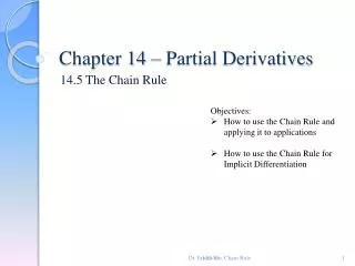
Constrained Optimisation • A similar optimisation problem to the one above is when a firm wants to maximise output subject to input constraints. • For example if a firms production function is: • Q = f(K, L) • The firm is then constrained by the price of capital (Pk) and the price of labour (PL) and the total income (M) available to spend on these inputs. • The constraint would then be: • PkK + PLL + M • This is known as the firms cost constraint and is illustrated over.
Here the optimal combination of capital and labour is where the firms cost constraint is tangential to the isoquant. Note that combinations B and C are also viable options. However they lie on a lower isoquant and hence reflect lower levels of output than point A.
Lagrange Multipliers • Lagrange multipliers is a method for finding the local extremes of a function of several variables subject to one or more constraints • The method reduces a problem in ‘n’ variables with ‘k’ constraints to a solvable problem in ‘n+k’ variables with no constraints. • The method introduces a new scalar variable, the Lagrange multiplier, for each constraint and forms a linear combination involving the multipliers as coefficients.
LagrangeMultipliers • Consider the following objective function that you wish to maximise: • f(x,y) • Subject to the constraint: • (x,y) = M • Where identifies a function and M is a constant. • Lagrange multipliers can be used to solve this problem be defining a function from the information above: • g(x,y, ,l) = f(x,y) + l(M - (x,y)) • To solve this function we find: • dg/dx, dg/dy and dg/dl • We then set eqch partial derivative equal to zero.
LagrangeMultipliers:Example • Use Lagrange multipliers to find the optimal value of: • x2 – 4xy + 16x • Subject to the constraint: • 4x + 2y = 8 • Re-arranging into the format above: • g(x,y, l) = x2 – 4xy + 16x + l(8-4x - 2y) • Finding the three partial derivatives: • dg/dx = 2x – 4y +16 -4l = 0 (1) • dg/dy = -4x -2 l = 0 (2) • dg/dl = 8-4x - 2y = 0 (3) • The solution to this is on the next slide.
LagrangeMultipliers:Example • Equation (2) x 2: • -8x -4 l = 0 (4) • Equation (1) - Equation (4): • (2x – 4y +16 -4l) - (-8x -4 l) = 0 • 10x – 4y + 16 = 0 (5) • Equation (3) x 2: • 16 – 8x – 4y = 0 (6) • Equation (5) – (6): • (10x – 4y + 16) – (16 – 8x – 4y) = 0 • 18x = 0, x =0 • Sub x=0 in (4), so l=0 • Sub x=0 in (5) or (6): • 10(0) – 4y + 16 = 0, y = 4
LagrangeMultipliers:Economic Applications • Consider the following utility function: • U(x1,x2) = 3x1x2 + 4x1 • The price of a unit of x1 is £3 and the price of x2 is £2. We will assume that the consumers income is £275. • The budget constraint is then: • 3x1 + 2x2 = 275 • Use the Lagrange multiplier approach to find the maximum value of utility. • g(x1,x2,l) = 3x1x2 + 4x1 + l(275 - 3x1 - 2x2) • dg/dx1 = 3x2 + 4 – 3l = 0 (1) • dg/dx2 = 3x1 – 2l = 0 (2) • dg/dl = 275 - 3x1 - 2x2 = 0 (3)
LagrangeMultipliers:Economic Applications • Equation (2) + (3): • (3x1 – 2l) + (275 - 3x1 - 2x2) = 0 • – 2l + 275 - 2x2 = 0 (4) • Re-arranging (4): • – 2l = - 275+ 2x2 • Multiplying by 3/2: • – 3l = -412.5+ 3x2 • And substituting in (1): • 3x2 + 4 – 3l = 0 • 3x2 + 4 + (-412.5+ 3x2) = 0 • 6x2 = 408.5 and so x2 = 68.08
LagrangeMultipliers:Economic Applications • Substituting x2 in (1): • 3(68.08) + 4 – 3l = 0 • 208.24 = 3l • l = 69.41 • Substituting l in (2): • 3x1 – 2(69.41) = 0 • x1 = 46.27 • Note you can check your results by using an online simultaneous equation solver such as the one at http://math.cowpi.com/systemsolver/3x3.html or use the techniques outlined in chapter 10.